AP Microeconomics Unit 1: Basic Economic Concepts Notes

Introduction

Scarcity creates tradeoffs, opportunity cost identifies what a choice displaces, and marginal reasoning compares the next benefit with the next cost.

The unit moves from a single choice to economy-wide production and then back to individual decisions. Keep the resource constraint explicit, state opportunity cost in units of the alternative forgone, and distinguish a productive-capacity change from a change in how existing capacity is used.

Allocation mechanisms coordinate choices through different information and incentive systems. Their modeled efficiency does not settle distribution, rights, or other social goals, so conclusions should stay within the assumptions of the model being used.

Scarcity and allocation

finite resources require a decision rule

Production possibilities

capacity, efficiency, and opportunity cost

Comparative advantage

relative cost and the range for beneficial trade

Marginal reasoning

compare the next benefit with the next cost

Reference

Formula and theorem sheet

Match each expression with the condition that makes it valid.

Current exam guidance: Aligned to the current 2026–27 AP Microeconomics framework. Every model identifies axes, assumptions, movement or shift, market structure, and the quantitative or welfare consequence.

1.1

Scarcity

Why does scarcity require a choice even when no money changes hands?

Short answer

A resource cannot serve all competing uses at once, so selecting one feasible use sacrifices the value of the next-best alternative.

Know firstRanking alternatives · Distinguishing a resource from the output it can produce

The constraint—not the price tag—creates the tradeoff

Scarcity exists whenever available time, labor, land, or capital cannot satisfy every competing use. It does not mean that an economy is poor or that every item is rare. A temporary shortage is a different idea: at a particular price, buyers want more than sellers offer. Scarcity remains because resources have alternative uses even after a shortage disappears.

Opportunity cost is the value of the best alternative that is not chosen. Suppose the same six labor-hours can produce a service valued at 15 units, equipment maintenance valued at 11, or record organization valued at 4. Choosing the service displaces maintenance, so its opportunity cost is 11 value units of maintenance. The third-ranked option is not added because it would not be selected if the first option vanished.

Economic model

Three uses of six labor-hours

Identify the chosen use and the single next-best forgone alternative.

Held constant: Each alternative uses all six labor-hours, and values are comparable within this one decision.
Time horizon: One work period.
Read the change: This is a choice ledger, not a curve. More available labor changes the feasible set; a changed ranking changes which feasible alternative is selected.

Selected value: 15
Opportunity cost: 11

Ranked feasible uses

Horizontal axis: Value from using all six hours (value units)
Vertical axis: Alternative

r1Servicer2Maintenancer3Records

Maintenance is the next-best forgone use.

OC(\text{service})=11\text{ value units of maintenance}

Service ranks first at 15 value units, maintenance second at 11, and records third at 4. Assigning all six hours to service has an opportunity cost of 11 value units of maintenance.

Read the model as a table

Three uses of six labor-hours values
Use of six hours	Value units	Role
Service	15	selected
Maintenance	11	next-best forgone
Records	4	other alternative

Find an opportunity cost

Hold the scarce resource constant.
List only feasible competing uses.
Rank the alternatives using the stated criterion.
Report the value and units of the highest-ranked rejected option.

Keep these three ideas

Scarcity is a persistent constraint; a shortage is a market condition at a price.
Opportunity cost is the next-best alternative forgone.
A choice can have an opportunity cost even when its money price is zero.

1.2

Resource Allocation and Economic Systems

How do different economic systems decide what, how, and for whom to produce?

Short answer

They use different combinations of prices, plans, rules, customs, and public provision to transmit information and assign scarce resources.

Know firstScarcity · Incentives · Opportunity cost

An allocation system links information to a decision

Every system must answer what to produce, how to produce it, and who receives it. A decentralized market uses prices, property rules, and exchange: bids communicate willingness and ability to pay, while expected profit changes suppliers’ incentives. An administrative system can rank requests using an announced rule such as medical urgency. Custom, household production, regulation, and public provision can also guide decisions.

Real economies mix these mechanisms. A clinic might reserve some hours for urgent cases and allocate the remainder through scheduled fees. The choice of mechanism affects what information matters, who bears costs, and how quickly the allocation responds. No label guarantees efficiency or equity. Market power, external effects, public goods, and missing information can weaken a market result; a plan can face information, incentive, and implementation limits.

Economic model

Allocation rules distribute the same capacity differently

Connect each mechanism to its information channel while holding total resources fixed.

Held constant: The same ten hours are distributed in every row; the categories are synthetic and mutually exclusive.
Time horizon: One clinic scheduling period.
Read the change: The visual compares decision rules rather than curve shifts. Changing the rule reallocates the fixed ten hours; expanding staff would change the resource constraint.

Price-bid total: 10
Need-rule total: 10
Mixed-rule total: 10

Price bidsNeed ruleReserved + scheduled

Horizontal axis: Rule–appointment category
Vertical axis: Clinic-hours allocated

Codes pair each rule (B, N, or M) with routine, urgent, or preventive appointments (R, U, or P).

h_{routine}+h_{urgent}+h_{preventive}=10

Each rule distributes exactly ten clinic-hours. Price bids assign 7, 2, and 1 hours; a need rule assigns 2, 6, and 2; the mixed rule assigns 4, 4, and 2 to routine, urgent, and preventive care.

Read the model as a table

Allocation rules distribute the same capacity differently values
Rule	Primary information	Routine hours	Urgent hours	Preventive hours	Total
Price bids	willingness and ability to pay	7	2	1	10
Need rule	medical priority	2	6	2	10
Reserved + scheduled	priority plus price/time slots	4	4	2	10

Analyze an allocation rule without relying on labels

Identify the decision maker.
Name the information used to rank requests.
Explain the incentive created by the rule.
Check whether the resource total is respected.
State an objective or effect the mechanism leaves unmeasured.

Keep these three ideas

Economic systems coordinate what, how, and for whom to produce.
Prices, plans, customs, and rules carry different information and incentives.
A modeled allocation result does not settle whether the distribution is fair.

1.3

Production Possibilities Curve

What can a production possibilities curve reveal about capacity and opportunity cost?

Short answer

By marking current maximum output combinations, a PPC shows feasibility and the amount of one output surrendered for another.

Know firstScarcity · Coordinate graphs · Slope with labeled units

Location answers feasibility; slope answers cost

A point on the PPC uses current resources productively to reach a maximum combination. A point inside is attainable but leaves resources idle or poorly assigned. A point outside is not currently feasible. Moving along the frontier changes the output mix; it does not change capacity. The choice of which frontier point to produce requires preferences or another social criterion that the graph does not supply.

Opportunity cost of horizontal-axis output is $|\Delta y/\Delta x|$ units of vertical output. Along the authored frontier, raising $x$ from 0 to 2 sacrifices 3 units of $y$ , or 1.5 $y$ per $x$ . The next two moves cost 2 and then 3 $y$ per $x$ . The increasing cost is consistent with resources becoming less suited to the expanding activity. A technology improvement specific to $x$ can extend the right side while leaving the $y$ intercept unchanged.

Economic model

Capacity, feasibility, and rising opportunity cost

Distinguish points from shifts and calculate segment opportunity costs.

Held constant: Resources and technology remain constant on the current PPC; output is measured per period.
Time horizon: Current capacity, with a comparison to an x-specific technology improvement.
Read the change: Changing the output mix moves along the PPC. Underusing resources moves inside it. A resource or technology change shifts some or all of the frontier.

First segment cost: 1.5 Y per X
Second segment cost: 2 Y per X
Third segment cost: 3 Y per X

Current PPCAfter X-specific technology

Horizontal axis: Good X (units per period)
Vertical axis: Good Y (units per period)

1interior2currently infeasible

The technology change expands X capacity without moving the Y intercept.

OC_X=\left|\frac{\Delta Y}{\Delta X}\right|

The current PPC begins at a Y-intercept of 14 and ends at an X-intercept of 6. Its first three segment costs rise from 1.5 to 2 to 3 units of Y per X. X-specific technology keeps the Y-intercept at 14 and extends the X-intercept to 7.5. The point 2 and 8 is interior.

Read the model as a table

Capacity, feasibility, and rising opportunity cost values
Record	X	Y	Meaning
Current PPC	0	14	unchanged Y-intercept
Current PPC	2	11	cost from prior point: 1.5 Y/X
Current PPC	4	7	cost: 2 Y/X
Current PPC	5	4	cost: 3 Y/X
Current PPC	6	0	current X-intercept
Technology PPC	7.5	0	expanded X-intercept
Interior point	2	8	attainable but productively inefficient
Outside point	4	11	currently infeasible

A worker installing electrical equipment in an airplane-production factory. — A production choice uses a finite combination of inputs
Labor, tools, floor space, and materials committed to one output cannot make another output at the same time. A production possibilities curve compresses those feasible choices into a two-good model.
Use this visual to see
Connect an abstract production frontier to the real inputs that make scarcity binding.
What it cannot show
The photograph shows one production process; it does not identify the economy-wide frontier, the opportunity-cost slope, or unused capacity.

Diagnose a PPC event

Locate the point relative to the current frontier.
If production changes on the frontier, calculate the slope with units.
If capacity changes, identify the affected resource or technology.
Decide whether the shift affects both outputs or one side more strongly.

Keep these three ideas

The PPC is a productive-capacity boundary.
Its absolute slope measures opportunity cost in named units.
Resource underuse changes the operating point; capacity changes shift the frontier.

1.4

Comparative Advantage and Trade

How do opportunity costs determine specialization and a mutually beneficial trade rate?

Short answer

The producer with the lower opportunity cost has comparative advantage, and both sides can gain when the exchange rate lies strictly between their internal costs.

Know firstPPC opportunity cost · Ratios and reciprocals · Consistent units

Relative sacrifice determines the assignment

Producer A can make 12 units of $x$ or 6 units of $y$ . One $x$ therefore costs A $6/12=0.5y$ . Producer B can make 5 units of $x$ or 10 units of $y$ , so one $x$ costs B $10/5=2y$ . A has comparative advantage in $x$ because A sacrifices less $y$ for each $x$ . The reciprocal costs show that B has comparative advantage in $y$ .

A rate of $1x$ for $1y$ lies between 0.5 and 2 $y$ per $x$ . A can make an $x$ at a cost of 0.5 $y$ and receive 1 $y$ for it; B can obtain an $x$ for 1 $y$ instead of sacrificing 2 $y$ internally. Trade can expand consumption possibilities even though it does not shift either producer’s PPC. Transport, adjustment, market power, and distribution can reduce or redirect the gains.

Economic model

Mutually beneficial terms of trade

Use consistent units to assign comparative advantage and test a proposed exchange rate.

Held constant: The two opportunity costs are stable, trade is voluntary, and transaction costs are zero.
Time horizon: One period of specialization and exchange.
Read the change: This interval does not depict a curve shift. A trade rate inside the interval changes attainable consumption; a productivity change would alter an endpoint.

A cost of 1X: 0.5Y
Exchange rate: 1Y per X
B cost of 1X: 2Y

Open interval for mutual gains

Horizontal axis: Units of Y exchanged for one X
Vertical axis: Comparison row

y1Terms-of-trade interval

1A endpoint21:1 trade3B endpoint

An endpoint leaves one producer indifferent; a strict interior rate can benefit both.

0.5Y<\text{terms for }1X<2Y

A sacrifices 0.5 units of Y for one X, while B sacrifices 2. A rate of one Y per X lies strictly between those internal costs, so A exports X and B exports Y in the simple model.

Read the model as a table

Mutually beneficial terms of trade values
Producer	Maximum X	Maximum Y	Cost of 1X	Cost of 1Y	Comparative advantage
A	12	6	0.5Y	2X	X
B	5	10	2Y	0.5X	Y
Proposed trade	—	—	1Y per X	1X per Y	inside both cost bounds

Workers transferring farm produce from a horse-drawn wagon to a truck for delivery to a city market in 1918. — Specialization matters because output can move to another market
Specialized producers gain access to a wider set of goods when exchange links farms, carriers, and buyers. The source of the gain is comparative advantage, not the age of the transport or the amount carried.
Use this visual to see
Place comparative advantage inside the exchange network that turns specialization into consumption possibilities.
What it cannot show
The scene cannot reveal either producer’s opportunity cost, the terms of trade, transaction costs, or how the gains are divided.

Keep the units fixed through the comparison

Calculate each producer’s cost of one X in Y per X.
Give X to the lower-cost producer.
Take reciprocals to check the assignment for Y.
Place a proposed rate strictly between the two same-unit costs.
Compare each producer’s trade cost with self-production.

Keep these three ideas

Comparative advantage belongs to the lower-opportunity-cost producer.
A mutually beneficial trade rate lies strictly between internal costs.
Aggregate gains from exchange do not guarantee equal individual gains.

1.5

Cost-Benefit Analysis

Which costs and benefits belong in a forward-looking decision?

Short answer

Compare incremental benefits with incremental opportunity costs from a stated perspective, while excluding costs that are already sunk.

Know firstOpportunity cost · Totals and differences · Private versus social effects

The baseline determines what is incremental

Cost-benefit analysis compares a decision with a specific alternative over a stated horizon. If adopting a future option adds 84 value units of benefit and 61 units of cost, its measured incremental net benefit is $84-61=23$ . A separate effect that cannot be valued credibly should be listed and discussed rather than silently treated as zero. Private analysis includes effects on the decision maker; social analysis also counts effects on others.

A sunk cost was incurred before the current decision and cannot be changed by either forward choice. A 30-unit study fee already paid does not belong on only one side of the new comparison. Future maintenance, forgone time, or environmental harm may belong because the choice can still alter them. A positive net-benefit total is conditional on the chosen perspective and measurement; it does not override legal rights, distribution, uncertainty, or consent.

Economic model

Forward effects of one option

Compute net benefit while keeping sunk and unpriced effects visible but separate.

Held constant: Benefit and future cost use a common value scale; the sunk 30-unit payment is identical under both forward alternatives.
Time horizon: Future effects of the current choice.
Read the change: This is an incremental ledger, not a market graph. A changed future consequence changes net benefit; a sunk payment does not change the forward difference.

Future benefit: 84
Future cost: 61
Incremental net benefit: 23
Excluded sunk payment: 30

Value ledger

Horizontal axis: Decision component
Vertical axis: Value units

x1Future benefit

The 30-unit payment stays visible for context but is excluded from the forward subtraction.

NB_{incremental}=84-61=23

The option adds 84 value units of future benefit and 61 of future cost, leaving 23 of measured incremental net benefit. A prior 30-unit payment is sunk and does not change the forward comparison.

Read the model as a table

Forward effects of one option values
Item	Value units	Forward decision treatment
Additional benefit	84	include
Additional opportunity cost	61	include
Measured net benefit	23	benefit minus cost
Previously paid study cost	30	exclude as sunk
Unpriced outside harm	not assigned zero	list and assess separately

Build a defensible comparison

State the decision, baseline, perspective, and horizon.
Include consequences that differ between the alternatives.
Exclude costs that cannot be changed now.
Keep nonmonetized effects visible.
Compute net benefit, then state important limits outside the total.

Keep these three ideas

Incremental net benefit compares a choice with its baseline.
Sunk costs do not change a forward-looking decision.
Unpriced effects should be identified rather than assigned an automatic value of zero.

1.6

Marginal Analysis and Consumer Choice

How should a consumer allocate a limited budget across goods?

Short answer

Compare marginal utility per dollar for the next affordable units and reallocate spending until no feasible switch raises total utility.

Know firstBudget constraints · Marginal versus total values · Opportunity cost

A dollar should go where its next payoff is greatest

Marginal utility is the added satisfaction from the next unit. Because goods have different prices, raw marginal utilities are not directly comparable. The useful measure is $MU/P$ : the additional utility obtained per dollar spent. For divisible goods at an interior optimum with the budget exhausted, the last units satisfy $MU_x/P_x=MU_y/P_y$ . If one ratio is higher, shifting a dollar toward that good can raise total utility.

Whole units can prevent exact ratio equality. With the authored schedules and a budget of 12, two units of $x$ and two of $y$ cost $2(2)+4(2)=12$ and generate $18+14+32+20=84$ utility units. Replacing the second $y$ with the third and fourth units of $x$ gives up 20 utility and adds only $10+6=16$ . The switch lowers utility by 4, so the bundle remains best among the feasible authored combinations. Utility is an individual ranking tool, not a measure of need or moral worth.

Economic model

Marginal utility per dollar by unit

Show why affordability and declining next-unit returns determine the selected bundle.

Held constant: Prices, budget, and this consumer’s marginal-utility schedules are fixed; units are indivisible.
Time horizon: One budget period.
Read the change: This is a marginal schedule rather than supply and demand. A change in price rescales MU per dollar; moving to another unit follows the existing schedule.

Cost of 2X + 2Y: 12 currency units
Total utility: 84
Utility from swap: −4

Good X: MU per currency unitGood Y: MU per currency unit

Horizontal axis: Unit number purchased
Vertical axis: Marginal utility per currency unit

1second X chosen2second Y chosen

Whole-unit affordability can prevent exact equality of the final ratios.

\frac{MU_x}{P_x}\quad\text{compared with}\quad\frac{MU_y}{P_y}

Good X has marginal utility per dollar values 9, 7, 5, and 3. Good Y has values 8, 5, and 2. With prices 2 and 4 and budget 12, the best authored whole-unit bundle is two X and two Y with utility 84.

Read the model as a table

Marginal utility per dollar by unit values
Unit	MU of X	MU/P for X at price 2	MU of Y	MU/P for Y at price 4
1	18	9	32	8
2	14	7	20	5
3	10	5	8	2
4	6	3	—	—
Chosen bundle	2 units	cost 4	2 units	cost 8

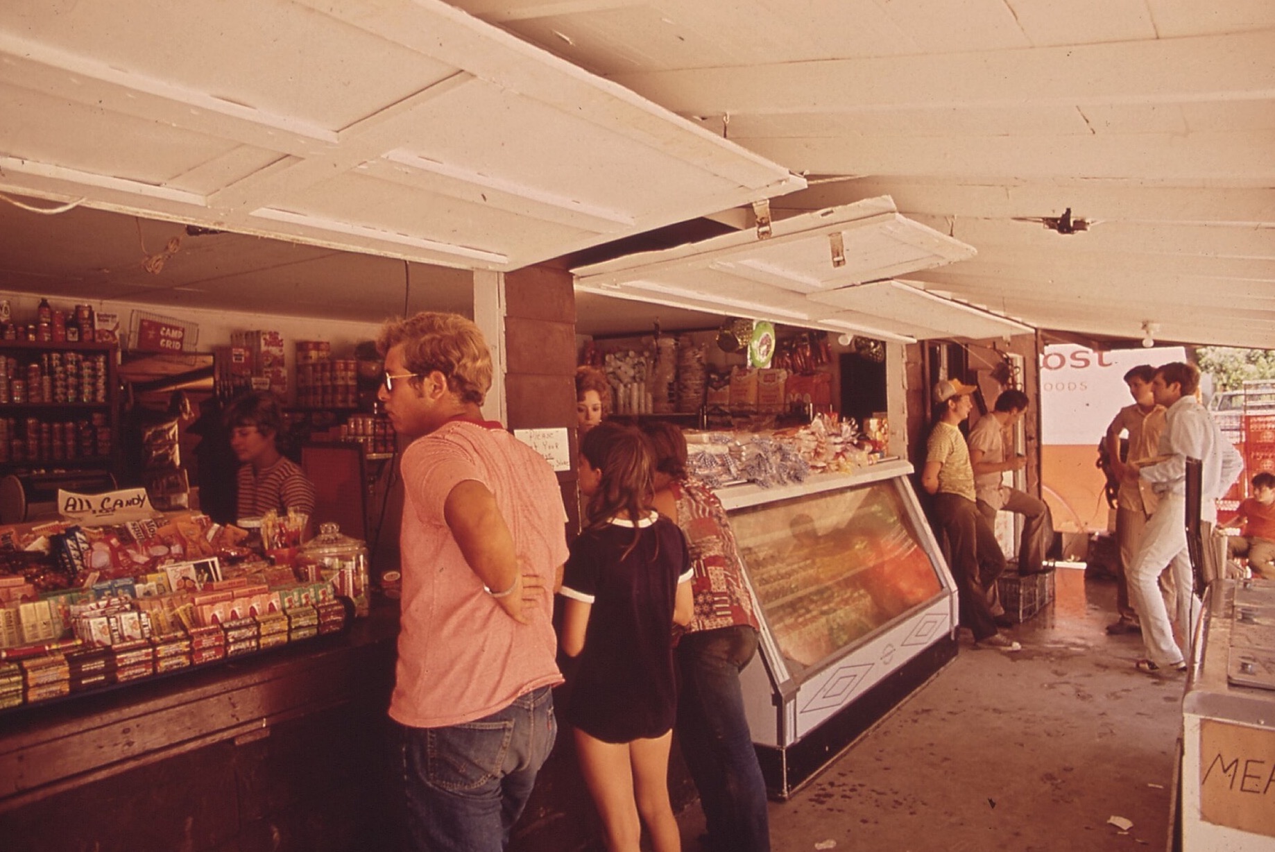
Shoppers choosing among groceries and other goods at a park store in Texas in 1972. — A budget turns preference into a constrained choice
A shopper compares the extra satisfaction from another unit with its price and with the alternatives that spending would displace. Consumer choice is therefore marginal and constrained, not a simple ranking of favorite goods.
Use this visual to see
Connect marginal utility per dollar to a setting where many affordable and unaffordable combinations compete for one budget.
What it cannot show
The photograph does not disclose any shopper’s income, prices faced, utility, quantities selected, or whether the final bundle is optimal.

Allocate a discrete budget

Compute marginal utility per dollar for each next unit.
Select the highest affordable next ratio.
Update the remaining budget after every unit.
Compare feasible swaps around the candidate bundle.
Stop when no affordable reallocation increases total utility.

Keep these three ideas

Marginal utility per dollar, not raw marginal utility, guides allocation.
An interior divisible optimum tends toward equal last-unit ratios.
Indivisibility and corners require a feasibility check rather than forced equality.

Cumulative review

Basic economic concepts review

Every model in this unit begins with a feasible set and a choice. Identify the constraint, the next-best alternative, the decision rule, and the conclusion the model cannot establish on its own.

Recognize immediately

Name the next-best alternative rather than adding every rejected option.
Separate movement inside a PPC from a shift in productive capacity.
Calculate comparative advantage with opportunity cost in matching units.
Exclude sunk costs from forward-looking marginal decisions.
Check affordability and corner solutions before imposing equal marginal-utility ratios.

Introduction

Formula and theorem sheet

The constraint—not the price tag—creates the tradeoff

Find an opportunity cost

Keep these three ideas

An allocation system links information to a decision

Analyze an allocation rule without relying on labels

Keep these three ideas

Location answers feasibility; slope answers cost

A production choice uses a finite combination of inputs

Diagnose a PPC event

Keep these three ideas

Relative sacrifice determines the assignment

Specialization matters because output can move to another market

Keep the units fixed through the comparison

Keep these three ideas

The baseline determines what is incremental

Build a defensible comparison

Keep these three ideas

A dollar should go where its next payoff is greatest

A budget turns preference into a constrained choice

Allocate a discrete budget

Keep these three ideas

Basic economic concepts review

Recognize immediately

Practice AP Microeconomics in the real test engine.