AP Physics C: Mechanics Unit 1: Kinematics Notes

Introduction

Kinematics uses vector functions, derivatives, and definite integrals to describe motion before identifying the forces that produce it.

Start with a frame, origin, axes, clock, and point-particle model. Position is a vector function of time. Velocity is its derivative, acceleration is the derivative of velocity, and initial conditions fix the constants created by integration.

The same motion can appear as a parametric path, component equations, graphs, or a table. A valid solution keeps the coordinate choices and time domain consistent while moving among those representations.

Vectors

separate magnitude from signed components

Derivatives

extract instantaneous velocity and acceleration

Integrals

accumulate displacement and velocity change

Frames and components

compare observers and solve multidimensional motion

Current exam guidance: Aligned to the current 2026–27 AP Physics C: Mechanics framework, with calculus-based modeling, derivations, experimental reasoning, and explicit assumptions.

1.1

Scalars and Vectors

How do components preserve a vector’s magnitude and direction?

Short answer

Components are signed projections on chosen axes; they change when the axes rotate, while the physical vector and its magnitude do not.

Know firstAlgebra · Right-triangle trigonometry · Three-dimensional coordinates

A vector is more than its length

A scalar has magnitude and units but no direction: distance and speed are scalars, while displacement, velocity, and acceleration are vectors. Write $\vec A=A_x\hat i+A_y\hat j+A_z\hat k$ . The unit vectors name axis directions and are dimensionless; the components carry the units and signs. Its magnitude is $|\vec A|=\sqrt{A_x^2+A_y^2+A_z^2}$ . Dividing by that magnitude gives $\hat A=\vec A/|\vec A|$ .

Vector addition is componentwise because each axis projection adds independently. Opposite components can cancel even when both vectors are large. Rotating the coordinate system changes $(A_x,A_y,A_z)$ but preserves $|\vec A|$ , so magnitude invariance is a strong error check.

Physics model

A component carries sign; magnitude does not

Move a one-dimensional vector endpoint and compare its signed component with its nonnegative magnitude. At zero, the vector has no direction.

Vector component3 m

Component: 3 m
Magnitude: 3 m
Direction: positive

originsigned axiscomponent vector

\vec A=A_x\hat{\mathbf i}

Read this figure without the graphic

Move a one-dimensional vector endpoint and compare its signed component with its nonnegative magnitude. At zero, the vector has no direction.

Current quantity	Value
Component	3 m
Magnitude	3 m
Direction	positive
Model relation	$\vec A=A_x\hat{\mathbf i}$

Resolve and recombine one vector

System: A directed displacement in three dimensions.
Frame: Fixed Cartesian axes with orthonormal $\hat i$ , $\hat j$ , and $\hat k$ .
Assumptions: Components use one common coordinate system.
Givens: $\vec A=3\hat i-4\hat j+12\hat k$ .

Square and add the components: $|\vec A|^2=3^2+(-4)^2+12^2=169$ .
Take the nonnegative square root: $|\vec A|=13$ .
Divide every component by 13 to obtain $\hat A$ .
Check $|\hat A|^2=(9+16+144)/169=1$ .

Result

\hat A=\frac{3}{13}\hat i-\frac{4}{13}\hat j+\frac{12}{13}\hat k

Units:

\vec A

has its physical units;

\hat A

is dimensionless.

Boundary cases

The zero vector has magnitude zero and no unique direction.
$|\vec A+\vec B|$ is generally not $|\vec A|+|\vec B|$ .

The component triple three, negative four, twelve forms a length-thirteen vector and normalizes to a unit vector.

Keep each quantity distinct

Quantity	Meaning	Can be negative?
$A_x$	signed projection on the x-axis	yes
$\|\vec A\|$	vector magnitude	no
$\hat A$	dimensionless direction	components may be
$\vec A+\vec B$	componentwise resultant	components may be

Audit a vector calculation

Declare the axes and units.
Resolve every vector in the same basis.
Add or subtract matching components.
Recombine only after the component algebra is complete.
Check magnitude, quadrant, and units.

Keep these three ideas

Components depend on the chosen axes.
Magnitude is invariant under an axis rotation.
Unit vectors specify direction and carry no physical units.

1.2

Displacement, Velocity, and Acceleration

How do derivatives and integrals connect position, velocity, and acceleration?

Short answer

Velocity and acceleration are successive time derivatives of position, while definite integrals recover changes once initial conditions are supplied.

Know firstVector components · Derivatives · Definite integrals

Motion is a chain of rates and accumulated changes

Model the moving object as a point particle whose position $\vec r(t)$ is measured from a chosen origin. Over $\Delta t$ , displacement is $\Delta\vec r$ , average velocity is $\Delta\vec r/\Delta t$ , and average acceleration is $\Delta\vec v/\Delta t$ . Taking the interval limit gives $\vec v=d\vec r/dt$ and $\vec a=d\vec v/dt$ . Speed is the scalar $|\vec v|$ .

Integration reverses differentiation only after physical initial data are included: $\vec v(t)=\vec v(t_0)+\int_{t_0}^{t}\vec a(s)\,ds$ and $\vec r(t)=\vec r(t_0)+\int_{t_0}^{t}\vec v(s)\,ds$ . From $t_0$ to $t_1$ , displacement is $\int_{t_0}^{t_1}\vec v\,dt$ , while distance traveled is $\int_{t_0}^{t_1}|\vec v|\,dt$ . Their magnitudes agree only when velocity keeps one fixed direction without reversing.

Physics model

Derivatives describe the instantaneous motion state

Move along a planar trajectory and compare its position, velocity, and acceleration vectors at one instant.

Time1 s

Position: $\langle-2,2\rangle$ m
Velocity: $\langle0,4\rangle$ m/s
Acceleration: $\langle6,4\rangle$ m/s²

trajectoryvelocity vectoracceleration vector

\begin{aligned}\vec r&=(t^3-3t)\hat{\mathbf i}+2t^2\hat{\mathbf j}\\ \vec v&=\frac{d\vec r}{dt},\qquad \vec a=\frac{d^2\vec r}{dt^2}\end{aligned}

Read this figure without the graphic

Move along a planar trajectory and compare its position, velocity, and acceleration vectors at one instant.

Current quantity	Value
Position	$\langle-2,2\rangle$ m
Velocity	$\langle0,4\rangle$ m/s
Acceleration	$\langle6,4\rangle$ m/s²
Model relation	$\begin{aligned}\vec r&=(t^3-3t)\hat{\mathbf i}+2t^2\hat{\mathbf j}\\ \vec v&=\frac{d\vec r}{dt},\qquad \vec a=\frac{d^2\vec r}{dt^2}\end{aligned}$

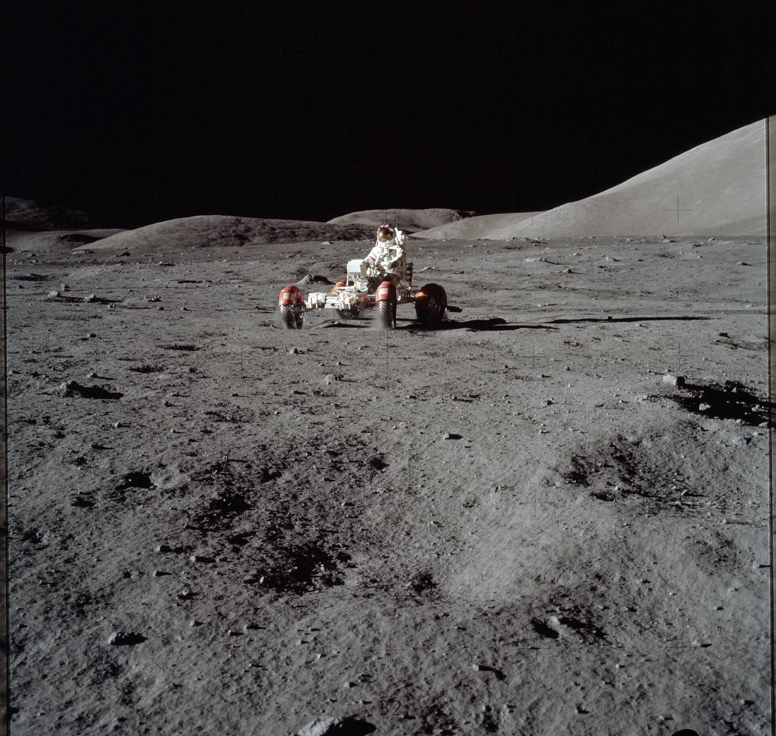
Apollo 17 astronaut Eugene Cernan drives the Lunar Roving Vehicle across the lunar surface. — Motion becomes data only after position is paired with time
The rover has a position in a chosen lunar coordinate system at each instant. A sequence of timed positions—not the single photograph—would let an analyst calculate velocity and acceleration.
Use this visual to see
Connect position, velocity, and acceleration to a moving physical system.
What it cannot show
The single frame establishes the rover and terrain but supplies no coordinate origin, scale, timestamps, velocity vector, or acceleration vector.

Differentiate a vector trajectory componentwise

System: A point particle following a smooth planar path.
Frame: Fixed inertial Cartesian frame.
Assumptions: $\vec r(t)$ is twice differentiable on the interval.
Givens: $\vec r(t)=(t^3-3t)\hat i+2t^2\hat j$ metres.

Differentiate each component once to find velocity.
Differentiate velocity once to find acceleration.
At $t=1\ \mathrm{s}$ , evaluate both velocity components before taking magnitude.

Result

\vec v=(3t^2-3)\hat i+4t\hat j,\qquad \vec a=6t\hat i+4\hat j

Units: Position is in m, velocity in m/s, and acceleration in m/s².

Boundary cases

$v_x(1)=0$ while $\vec v(1)=4\hat j\ \mathrm{m/s}$ .
A corner in $\vec r(t)$ may make instantaneous velocity undefined.

Differentiating each coordinate produces a vertical velocity of four metres per second at one second even though the horizontal velocity is zero.

Formula

Use definite integrals to preserve initial data

\displaystyle \Delta\vec r=\int_{t_0}^{t_1}\vec v\,dt,\qquad \Delta\vec v=\int_{t_0}^{t_1}\vec a\,dt

Signed vector areas accumulate displacement and velocity change.

Use when: The integrands must be integrable over the chosen interval and described in one frame.
Do not assume: Replacing $\vec v$ by $|\vec v|$ changes displacement into distance.

Move through the derivative chain

Write every component as a function of the same time.
Differentiate componentwise to move from position to velocity to acceleration.
Integrate with explicit bounds or restore constants from initial conditions.
Use $|\vec v|$ only when speed or distance is required.
Check continuity and units at interval boundaries.

Keep these three ideas

Velocity and acceleration are vector derivatives.
Initial conditions select the physical antiderivative.
Integrating speed gives distance; integrating velocity gives displacement.

1.3

Representing Motion

How do graphs, equations, and motion diagrams encode the same calculus relationships?

Short answer

Successive graph slopes give velocity and acceleration, while signed areas reverse those changes; equations must use the acceleration model that actually applies.

Know firstKinematic derivatives · Signed area · Initial conditions

Translate the axes before reading the shape

The slope of an $x$ – $t$ graph is $v_x$ ; the slope of a $v_x$ – $t$ graph is $a_x$ . Signed area under velocity gives displacement, and signed area under acceleration gives velocity change. A position graph is not a drawing of the spatial path, and graph height never changes meaning simply because the curve looks steep.

For constant $a_x$ , integration gives $v_x=v_{x0}+a_xt$ , $x=x_0+v_{x0}t+\tfrac12a_xt^2$ , and $v_x^2=v_{x0}^2+2a_x(x-x_0)$ . Near Earth, use $g=10\ \mathrm{m/s^2}$ unless another value is supplied. If acceleration varies with time, integrate $a_x(t)$ ; if it depends on position, use $a_x=v_x\,dv_x/dx$ . Model choice comes before algebra.

Physics model

Slope and signed area connect motion graphs

Trace one instant across three graphs; the tangent to position matches velocity, and velocity area gives displacement.

Time1 s

Position: 3 m
Velocity: 2 m/s
Acceleration: 2 m/s²
Displacement from 0: 2 m

positionvelocityaccelerationslope and area link

\begin{aligned}x&=t^3-2t^2+3t+1\\ v&=3t^2-4t+3,\qquad a=6t-4\end{aligned}

Read this figure without the graphic

Trace one instant across three graphs; the tangent to position matches velocity, and velocity area gives displacement.

Current quantity	Value
Position	3 m
Velocity	2 m/s
Acceleration	2 m/s²
Displacement from 0	2 m
Model relation	$\begin{aligned}x&=t^3-2t^2+3t+1\\ v&=3t^2-4t+3,\qquad a=6t-4\end{aligned}$

Integrate a changing acceleration exactly

System: A point particle constrained to one axis.
Frame: Inertial frame with fixed $+x$ .
Assumptions: $a(t)=(6\ \mathrm{m/s^3})t-4\ \mathrm{m/s^2}$ is continuous for $0\le t\le2\ \mathrm{s}$ .
Givens: $v(0)=3\ \mathrm{m/s}$ and $x(0)=1\ \mathrm{m}$ .

Integrate acceleration from 0 to $t$ : $v(t)=v(0)+\int_0^t a(s)\,ds$ .
With $t$ measured in seconds, the numerical form is $v(t)=3t^2-4t+3$ .
Integrate velocity from 0 to $t$ and add the initial position.
Differentiate the result twice to check the original acceleration.

Result

x(t)=t^3-2t^2+3t+1

Units: In the displayed numerical polynomials, time is entered in seconds; the resulting velocity is in m/s and position in m.

Boundary cases

The usual constant- $a$ formulas do not span this interval.
Here $v(t)>0$ for all real $t$ because its discriminant is negative; on this fixture, distance therefore equals displacement.

Two definite integrations turn the linear acceleration into a quadratic velocity and cubic position while preserving both initial conditions.

Read slopes and areas by axis labels

Graph	Slope	Signed area
$x$ versus $t$	$v_x$	no standard kinematic quantity
$v_x$ versus $t$	$a_x$	$\Delta x$
$a_x$ versus $t$	rate of acceleration change	$\Delta v_x$

Choose the motion relation

Identify what varies and what remains constant.
Use slopes for instantaneous rates and definite areas for accumulated changes.
If $a$ depends on $t$ , integrate in time.
If $a$ depends on $x$ , consider $a=v\,dv/dx$ .
Apply initial conditions and differentiate to verify.

Keep these three ideas

Graph slopes move forward through the derivative chain.
Signed areas accumulate motion changes.
Variable acceleration must be integrated with the correct independent variable.

1.4

Reference Frames and Relative Motion

Why can inertial observers disagree on velocity but agree on acceleration?

Short answer

A constant frame velocity adds to every measured velocity, but its derivative is zero, so Galilean-related inertial frames assign the same acceleration.

Know firstVector addition · Time derivatives · Subscript notation

Connect positions before differentiating

If frame B translates relative to frame A while their axes remain parallel, position vectors obey $\vec r_{P/A}=\vec r_{P/B}+\vec r_{B/A}$ . Differentiation gives the corresponding velocity relation. When $\vec v_{B/A}$ is constant, differentiating again removes the frame offset and both observers obtain the same acceleration.

Subscripts prevent sign errors: $\vec v_{A/B}=-\vec v_{B/A}$ . This treatment assumes axes that do not rotate and origins with constant relative velocity. An accelerating or rotating observer needs extra terms, so it is not related by this simple Galilean transformation.

Physics model

A Galilean transformation changes velocity, not acceleration

Change the inertial observer speed and compare the object velocity assigned in each frame.

Frame speed2 m/s

Laboratory velocity: 6 m/s
Moving-frame velocity: 4 m/s
Acceleration in both frames: unchanged

laboratory framemoving framerelative velocity

\begin{aligned}x^{\prime}&=x-Vt\\ v^{\prime}&=v-V,\qquad a^{\prime}=a\end{aligned}

Read this figure without the graphic

Change the inertial observer speed and compare the object velocity assigned in each frame.

Current quantity	Value
Laboratory velocity	6 m/s
Moving-frame velocity	4 m/s
Acceleration in both frames	unchanged
Model relation	$\begin{aligned}x^{\prime}&=x-Vt\\ v^{\prime}&=v-V,\qquad a^{\prime}=a\end{aligned}$

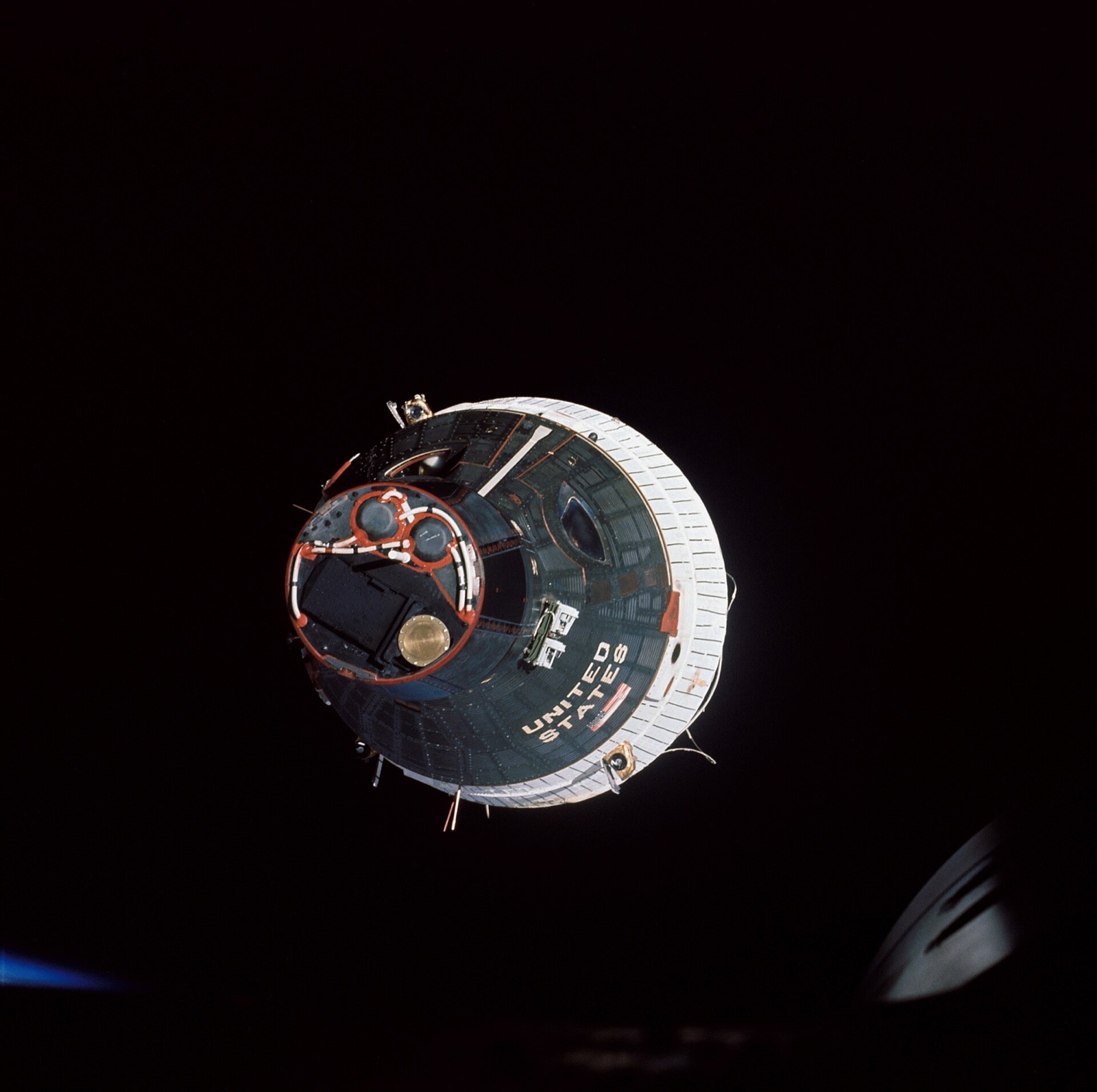
Gemini 7 photographed from Gemini 6 during the first crewed spacecraft rendezvous. — Rendezvous depends on relative position and velocity
The two spacecraft can move rapidly around Earth while changing position only slowly relative to each other. A frame attached to either capsule subtracts the frame velocity from both motion descriptions.
Use this visual to see
Connect relative velocity to an actual orbital rendezvous.
What it cannot show
Perspective does not provide the spacecraft separation, relative speed, or orbital elements; those require measurements in a stated reference frame.

Build a velocity chain

System: Particle P observed from translating frame B and laboratory frame A.
Frame: Two nonrotating inertial Cartesian frames.
Assumptions: $\vec v_{B/A}$ is constant.
Givens: $\vec v_{B/A}=(4,0)\ \mathrm{m/s}$ and $\vec v_{P/B}=(-1,3)\ \mathrm{m/s}$ .

Write $\vec r_{P/A}=\vec r_{P/B}+\vec r_{B/A}$ .
Differentiate once.
Add matching components.
Differentiate once more and use $d\vec v_{B/A}/dt=0$ .

Result

\vec v_{P/A}=(3,3)\ \mathrm{m/s},\qquad \vec a_{P/A}=\vec a_{P/B}

Units: Frame and particle velocities use m/s; accelerations use m/s².

Boundary cases

An accelerating B frame has $\vec a_{P/A}=\vec a_{P/B}+\vec a_{B/A}$ .
Rotating axes require additional rotational terms.

Adding the frame velocity to the particle velocity gives three metres per second in both laboratory directions; constant frame motion does not alter acceleration.

What survives a Galilean frame change?

Quantity	Relation	Same in both frames?
position	$\vec r_{P/A}=\vec r_{P/B}+\vec r_{B/A}$	not generally
velocity	$\vec v_{P/A}=\vec v_{P/B}+\vec v_{B/A}$	not generally
acceleration	$\vec a_{P/A}=\vec a_{P/B}$	yes, for nonrotating frames with constant relative velocity

Keep the observer accounting visible

Define every subscript in words.
Connect the target frames through a vector chain.
Differentiate only after the position relation is correct.
Apply the inertial and nonrotating conditions.
Reverse one relation to check antisymmetry.

Keep these three ideas

Relative positions form a vector chain.
Constant relative velocity shifts measured velocities.
Nonrotating inertial frames agree on acceleration.

1.5

Motion in Two or Three Dimensions

How do component differential equations build one multidimensional trajectory?

Short answer

Integrate each acceleration component with its own initial data, then evaluate every component at the same time to reconstruct the particle’s path and velocity.

Know firstVector derivatives · Definite integrals · Parametric curves

Components evolve independently but share one clock

For $\vec a(t)=a_x(t)\hat i+a_y(t)\hat j$ , integrate each component separately. Initial velocity and position can differ by axis, but the common time variable reunites the components into $\vec r(t)$ . The velocity vector is tangent to the parametric path; acceleration points in the direction of velocity change and need not be tangent.

Ideal projectile motion is the special case $a_x=0$ and $a_y=-g$ . More general time-dependent acceleration remains solvable componentwise. Independence fails when an interaction such as drag depends on the full speed $|\vec v|$ , because then one component equation contains the others. AP Physics C: Mechanics requires quantitative analysis in two dimensions; three-dimensional motion is treated qualitatively.

Physics model

Vector calculus separates perpendicular motion

Advance a projectile while horizontal and vertical components evolve under one shared time parameter.

Time1 s

Horizontal velocity: 8 m/s
Vertical velocity: 2 m/s
Acceleration: $\langle0,-10\rangle$ m/s²

trajectoryvelocity componentsacceleration

\vec r(t)=\langle v_{0x}t,\ y_0+v_{0y}t-\tfrac12gt^2\rangle

Read this figure without the graphic

Advance a projectile while horizontal and vertical components evolve under one shared time parameter.

Current quantity	Value
Horizontal velocity	8 m/s
Vertical velocity	2 m/s
Acceleration	$\langle0,-10\rangle$ m/s²
Model relation	$\vec r(t)=\langle v_{0x}t,\ y_0+v_{0y}t-\tfrac12gt^2\rangle$

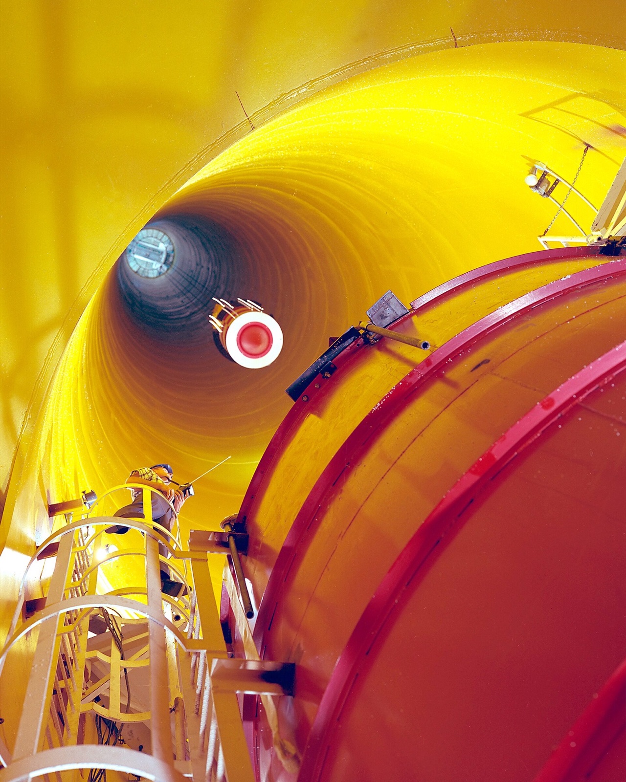
View upward through the tall cylindrical shaft of NASA’s Zero Gravity Facility. — A drop tower creates a controlled interval of free fall
An experiment package falls through the evacuated shaft so drag is greatly reduced. During the drop, the package and everything inside it accelerate together under gravity.
Use this visual to see
Show how an experimental apparatus isolates free-fall motion.
What it cannot show
The photograph establishes the long vertical shaft but does not show a drop trajectory, elapsed time, vacuum pressure, or measured acceleration.

Integrate nonuniform planar acceleration

System: A point particle moving in a plane.
Frame: Earth-fixed inertial approximation with $+y$ upward.
Assumptions: $a_x(t)=(2\ \mathrm{m/s^3})t$ , $a_y=-10\ \mathrm{m/s^2}$ , and drag is negligible.
Givens: $\vec v(0)=(4,6)$ m/s and $\vec r(0)=(0,1)$ m.

Integrate $a_x(t)$ and $a_y$ from zero to $t$ .
Add the two initial velocity components.
Integrate the resulting velocity components.
Add the two initial position components.

Result

\vec v=(t^2+4)\hat i+(6-10t)\hat j,\quad \vec r=\left(\frac{t^3}{3}+4t\right)\hat i+(1+6t-5t^2)\hat j

Units: In the numerical formulas, time is entered in seconds; position is returned in m and velocity in m/s.

Boundary cases

At $t=0.6$ s, $v_y=0$ but $v_x=4.36$ m/s.
Velocity-dependent drag couples the component equations.

Time integration produces a cubic horizontal coordinate and quadratic vertical coordinate; the particle keeps moving horizontally at its vertical apex.

Keep the component ledger aligned

Axis	Acceleration	Velocity	Position
x	$2t$	$t^2+4$	$t^3/3+4t$
y	$-10$	$6-10t$	$1+6t-5t^2$

Solve a vector initial-value problem

Declare axes and write each acceleration component.
Integrate using the matching initial velocity.
Integrate again using the matching initial position.
Apply one shared time or event condition.
Recombine components only for magnitude, direction, or path information.

Keep these three ideas

Integrate acceleration one component at a time.
All components describe the same particle at the same time.
Velocity is tangent to the path; acceleration need not be.

Cumulative review

Kinematics review

A complete kinematics model names its frame and domain, expresses motion componentwise, and uses derivatives or definite integrals without losing initial conditions.

Recognize immediately

Declare axes before assigning signs to components.
Differentiate position to obtain velocity and acceleration; integrate with initial conditions to reverse the process.
Use signed velocity area for displacement and integrate speed for distance.
Treat perpendicular component equations independently but evaluate them at the same time.

Introduction

A vector is more than its length

Resolve and recombine one vector

Boundary cases

Keep each quantity distinct

Audit a vector calculation

Keep these three ideas

Motion is a chain of rates and accumulated changes

Motion becomes data only after position is paired with time

Differentiate a vector trajectory componentwise

Boundary cases

Use definite integrals to preserve initial data

Move through the derivative chain

Keep these three ideas

Translate the axes before reading the shape

Integrate a changing acceleration exactly

Boundary cases

Read slopes and areas by axis labels

Choose the motion relation

Keep these three ideas

Connect positions before differentiating

Rendezvous depends on relative position and velocity

Build a velocity chain

Boundary cases

What survives a Galilean frame change?

Keep the observer accounting visible

Keep these three ideas

Components evolve independently but share one clock

A drop tower creates a controlled interval of free fall

Integrate nonuniform planar acceleration

Boundary cases

Keep the component ledger aligned

Solve a vector initial-value problem

Keep these three ideas

Kinematics review

Recognize immediately

Practice AP Physics C: Mechanics in the real test engine.