Now readingIntroduction
0%
AP Macroeconomics · Framework 2026-27
Unit 1

Basic Economic Concepts

Scarcity forces choices, opportunity cost measures the best forgone alternative, and markets coordinate choices through demand, supply, and equilibrium.

Exam weight
5–10%
Topics
6
production possibilities curve
Tradeoffs define the feasible setA downward-sloping, bowed production possibilities curve runs from high capital-goods output to high consumer-goods output. Its changing slope represents increasing opportunity cost.

Introduction

Scarcity forces choices, opportunity cost measures the best forgone alternative, and markets coordinate choices through demand, supply, and equilibrium.

This unit builds the vocabulary used throughout macroeconomics. Begin with a constraint: resources and time are limited. Then make the tradeoff visible with a production possibilities curve, compare opportunity costs to find comparative advantage, and use demand and supply to explain how decentralized market choices meet.

Keep positive analysis separate from judgment. Efficiency, equilibrium, and gains from trade describe what a model predicts under stated assumptions; they do not determine whether an allocation is fair or whether a policy is desirable.

01
Scarcity

choice and opportunity cost

02
Production possibilities

feasibility, efficiency, and growth

03
Comparative advantage

specialization and mutually beneficial terms of trade

04
Demand and supply

market equilibrium and adjustment

Formula and theorem sheet

Match each expression with the condition that makes it valid.

Current exam guidance: Aligned to the current 2026–27 AP Macroeconomics framework. Models identify their axes, assumptions, time horizon, movement or shift, and quantitative consequence.
1.1

Scarcity

Why does every economic choice have a cost?

Short answer

Resources have competing uses, so choosing one feasible alternative gives up the value of the next-best alternative.

Know firstRanking alternatives · Finite resources and time

Scarcity begins with competing uses

Scarcity means available resources cannot satisfy every competing use at once. It persists even in a wealthy economy and even when a particular item is plentiful. A shortage is different: it is a temporary gap between quantity demanded and quantity supplied at a given price. Scarcity is the underlying reason choices exist.

Opportunity cost is not every rejected option added together. It is the value of the best alternative that the choice displaces. If six labor-hours could produce a service worth 12 value units, maintenance worth 9, or filing worth 4, assigning the hours to service work gives up maintenance—the next-best option worth 9. Money can be part of a cost, but time and forgone output matter even when no payment occurs.

Economic model

Allocation of six labor-hours

Connect a chosen use to exactly one next-best forgone alternative.

Held constant
All alternatives use the same indivisible six labor-hours and values use one stated ranking criterion.
Time horizon
One allocation decision.
Read the change
This is a ranked-choice visual rather than a curve model; changing the resource constraint changes the feasible alternatives, while changing the ranking changes the chosen alternative.
Chosen value
12
Opportunity cost
9
Chosen: serviceNext best: maintenanceOther: filing
Allocation of six labor-hoursAll three alternatives require the same six labor-hours. Service ranks first at 12 value units, maintenance second at 9, and filing third at 4. Choosing service has an opportunity cost of 9, not 13.
Horizontal axis
Alternative
Vertical axis
Value from using all six hours (value units)
  • Opportunity cost = maintenance
OC(service)=value of maintenance=9OC(\text{service})=\text{value of maintenance}=9

All three alternatives require the same six labor-hours. Service ranks first at 12 value units, maintenance second at 9, and filing third at 4. Choosing service has an opportunity cost of 9, not 13.

Read the model as a table
Allocation of six labor-hours values
Use of six hoursValue unitsDecision role
Service12chosen
Maintenance9next-best forgone
Filing4other forgone

Name the displaced alternative

  1. List feasible alternatives that compete for the same resource.
  2. Rank them using the decision maker's stated criterion.
  3. Identify the chosen option.
  4. Report the next-best forgone option and its value with units.

Keep these three ideas

  • Scarcity is persistent; a shortage is market-specific and may be temporary.
  • Opportunity cost is the next-best alternative forgone.
  • A zero-dollar choice can still consume scarce time or resources.
1.2

Opportunity Cost and the Production Possibilities Curve (PPC)

What does a production possibilities curve reveal about an economy’s choices?

Short answer

A PPC separates attainable from unattainable output combinations and uses its slope to show the opportunity cost of producing more of one good.

Know firstScarcity · Slope as change in vertical divided by change in horizontal

The frontier is a capacity boundary

Every point on a PPC is a maximum attainable combination with current resources and technology. An interior point is attainable but leaves resources unemployed or misallocated. An exterior point is not attainable under the stated conditions. The frontier says nothing by itself about which efficient point society should prefer.

Moving right along the curve produces more of the horizontal-axis good and sacrifices some vertical-axis good. The absolute slope, ∣Δy/Δx∣|\Delta y/\Delta x|, is the opportunity cost of one additional unit of xx measured in units of yy. A straight frontier has constant opportunity cost. A bowed-out frontier has increasing opportunity cost because resources transferred toward one use become progressively less suited to it. More resources or better technology shift capacity; unemployment moves production inside the same frontier.

Economic model

Bowed-out production possibilities frontier

Show attainable regions and rising opportunity cost along one frontier.

Held constant
Resources, technology, and the production period remain fixed along the displayed frontier.
Time horizon
One current-capacity production period.
Read the change
Changing the output mix moves along the current PPC; changing productive resources or technology shifts the PPC.
First segment cost
1.5 consumer goods per capital good
Last segment cost
4 consumer goods per capital good
Current PPCattainable
Bowed-out production possibilities frontierThe frontier runs from 0 capital and 12 consumer goods to 5.5 capital and 0 consumer goods. Across the displayed segments, the cost of another capital good rises from 1.5 to 2 to 3 to 4 consumer goods.12
Horizontal axis
Capital goods (units per period)
Vertical axis
Consumer goods (units per period)
1attainable but inefficient2currently unattainable
  • Segments become steeper moving right
OCx=∣ΔyΔx∣OC_x=\left|\frac{\Delta y}{\Delta x}\right|

The frontier runs from 0 capital and 12 consumer goods to 5.5 capital and 0 consumer goods. Across the displayed segments, the cost of another capital good rises from 1.5 to 2 to 3 to 4 consumer goods.

Read the model as a table
Bowed-out production possibilities frontier values
Capital goodsConsumer goodsStatus
012efficient
29efficient
45efficient
52efficient
5.50efficient
27attainable interior
49unattainable
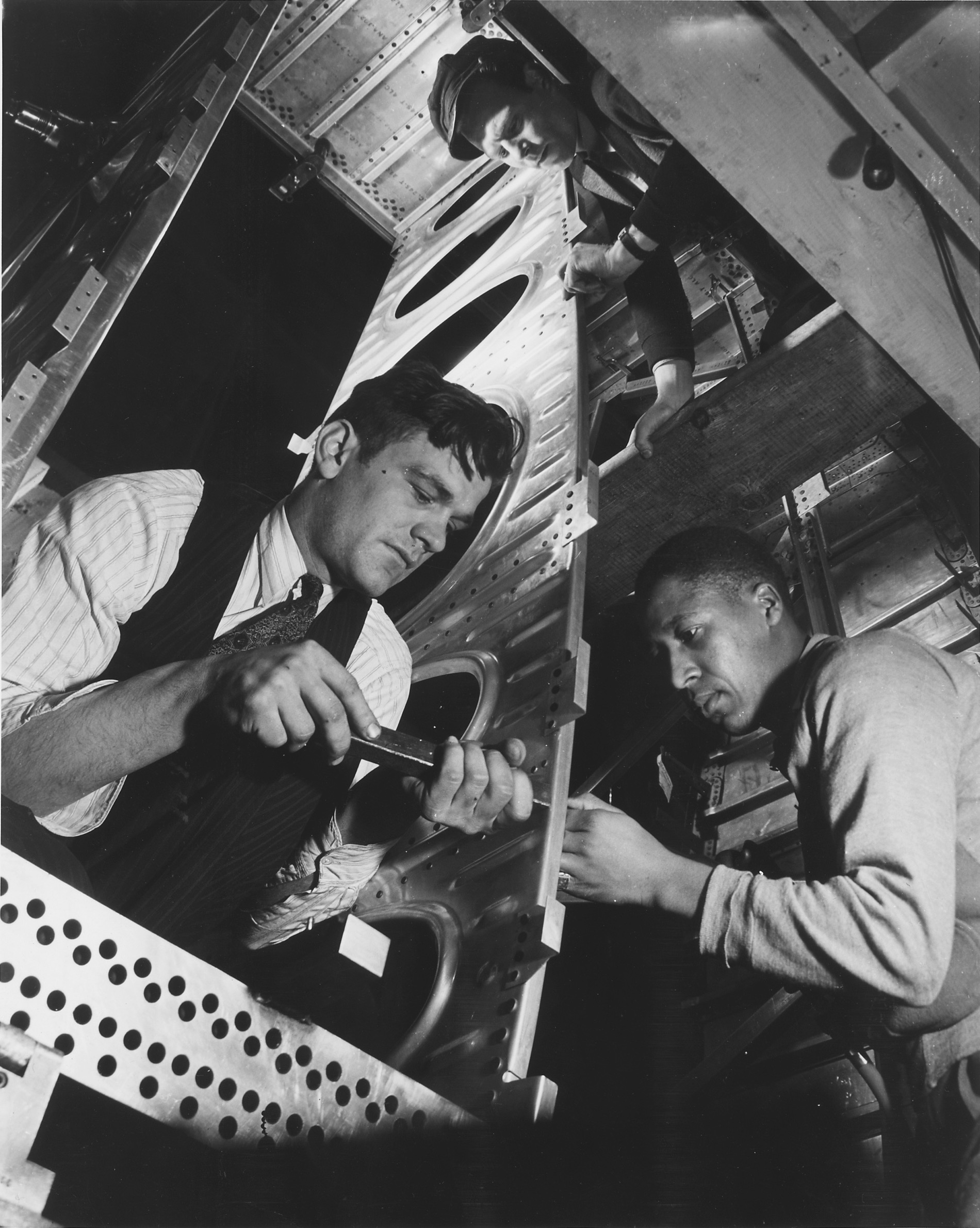
Economy in context
Three workers fastening metal components inside an aircraft frame at a bomber production plant, circa May 1942.

A production choice commits real resources

Labor, machinery, floor space, and materials committed to this production line cannot simultaneously produce another good. A production possibilities curve summarizes that tradeoff for an entire economy.

Use this visual to see
Connect an abstract production choice to finite labor and capital used in a specific production process.
What it cannot show
The photograph shows one factory, not the economy’s complete set of feasible combinations or the opportunity cost between two outputs.

Diagnose a PPC change

  1. Identify whether the point changes or the productive constraint changes.
  2. For a move along the frontier, calculate the forgone vertical output per added horizontal output.
  3. For a shift, name the resource or technology change.
  4. Allow one intercept to shift more than the other when the change is sector-specific.

Keep these three ideas

  • On-curve points are productively efficient; interior points are attainable but inefficient.
  • The PPC slope gives opportunity cost.
  • A capacity change shifts the frontier; resource underuse changes the operating point.
1.3

Comparative Advantage and Gains from Trade

How can two producers both gain from specialization and trade?

Short answer

Each producer specializes toward the good it can make at lower opportunity cost, then trades at a rate between the two opportunity costs.

Know firstOpportunity cost · Reciprocal rates · Production possibilities

Relative cost—not total output—determines specialization

Absolute advantage asks who can produce more with the same resources. Comparative advantage asks who gives up less of the other good. Producer A can make 8 units of xx or 4 of yy, so one xx costs A 0.5yy. Producer B can make 4xx or 8yy, so one xx costs B 2yy. A has comparative advantage in xx, while B has it in yy.

A trade rate of 1xx for 1yy lies between 0.5yy and 2yy per xx. A receives more yy through trade than it sacrifices to make an xx; B obtains an xx for less yy than internal production would cost. Trade expands consumption possibilities, not physical production by itself. Transport costs, adjustment unemployment, changing opportunity costs, and the distribution of gains can narrow the result.

Economic model

Two producers and one terms-of-trade interval

Separate absolute output from opportunity cost and display acceptable trade rates.

Held constant
Opportunity costs remain constant in the displayed range and transaction costs are omitted.
Time horizon
One production-and-trade period.
Read the change
This is an opportunity-cost interval rather than a market-curve shift; a rate strictly between internal costs creates scope for mutual gain.
A: cost of 1x
0.5y
B: cost of 1x
2y
Shown trade rate
1y per x
possible terms of trade
Two producers and one terms-of-trade intervalA gives up 0.5 units of y for one x and B gives up 2. A trade rate of one y per x sits strictly between those costs, so A exports x and B exports y.123
Horizontal axis
Units of y paid for one x
Vertical axis
Reference markers
1A internal cost; A is indifferent at this endpoint2trade rate that benefits both3B internal cost; B is indifferent at this endpoint
  • A strict interior rate can benefit both producers

0.5y<price of 1x<2y0.5y<\text{price of }1x<2y

A gives up 0.5 units of y for one x and B gives up 2. A trade rate of one y per x sits strictly between those costs, so A exports x and B exports y.

Read the model as a table
Two producers and one terms-of-trade interval values
ProducerMaximum xMaximum yCost of 1xComparative advantage
A840.5yx
B482yy
Trade2x exported by A2y exported by B1y per xboth can gain
Economy in context
Quay cranes lifting shipping containers beside a container ship at the Port of Savannah.

Specialization depends on a larger trading network

Ports connect specialized producers with buyers in other markets. Gains from trade still depend on relative opportunity costs and a mutually acceptable trading price—not simply on the volume of cargo moved.

Use this visual to see
Place comparative advantage inside the transportation network that makes large-scale exchange possible.
What it cannot show
Container traffic does not reveal either trading partner’s opportunity cost, terms of trade, distribution of gains, or environmental costs.

Build a comparative-advantage table

  1. Convert both producers into the same opportunity-cost units.
  2. Assign each good to the producer with the lower cost.
  3. State a terms-of-trade range strictly between the two costs.
  4. Check each producer against what receiving the import would cost internally.

Keep these three ideas

  • Comparative advantage means lower opportunity cost.
  • Terms of trade must lie between producers' internal costs.
  • Aggregate gains do not imply equal gains for every person.
1.4

Demand

What changes quantity demanded, and what changes demand itself?

Short answer

A change in the good’s own price moves along its demand curve; a change in another determinant shifts the entire demand schedule.

Know firstCoordinates and schedules · Holding other variables constant

Demand is a schedule, not one purchase amount

Demand pairs every possible own price with a quantity buyers are willing and able to purchase during a period. Quantity demanded is one point on that schedule. The usual inverse relationship reflects substitution toward alternatives and the reduced purchasing power of a higher price, with other influences held constant.

When the good's own price changes, the graph selects a different point on the same curve. Income, tastes, expectations, the prices of substitutes or complements, and the number of buyers shift the curve. Higher income shifts demand right for a normal good but left for an inferior good; those labels describe the direction of an income response, not quality. Market demand adds individual quantities at each common price.

Economic model

Original and expanded market demand

Link a schedule to its curve and distinguish a point change from a horizontal shift.

Held constant
Income, tastes, expectations, related prices, and buyer count remain fixed along D₁.
Time horizon
One market week.
Read the change
A change in the good's own price moves along demand; a change in a held-constant determinant shifts demand.
Original quantity at P=6
4
Expanded quantity at P=6
6
D₁D₂ after another buyer
Original and expanded market demandOriginal demand pairs prices 8, 6, 4, and 2 with quantities 2, 4, 6, and 8. Adding a buyer who demands two units at every price shifts each quantity right by two.12
Horizontal axis
Quantity demanded (units per week)
Vertical axis
Price (currency per unit)
1higher own price2lower own price
  • own-price change: move along D₁
  • buyer count rises: D₁ shifts to D₂
QDmarket(P)=∑iQD,i(P)Q_D^{market}(P)=\sum_i Q_{D,i}(P)

Original demand pairs prices 8, 6, 4, and 2 with quantities 2, 4, 6, and 8. Adding a buyer who demands two units at every price shifts each quantity right by two.

Read the model as a table
Original and expanded market demand values
PriceD₁ quantityD₂ quantity
824
646
468
2810

Use the axis test

  1. Name the variable that changed.
  2. If it is the good's own price on the vertical axis, move along demand.
  3. If it is a held-constant determinant, shift demand.
  4. Use the determinant's mechanism to choose left or right.
  5. Do not predict equilibrium price until supply is present.

Keep these three ideas

  • Demand is the full price–quantity schedule.
  • Own-price changes move along demand.
  • Income, preferences, expectations, related prices, and buyer count can shift demand.
1.5

Supply

What changes quantity supplied, and what changes supply itself?

Short answer

A change in the good’s own price moves along supply; a change in production conditions shifts the supply schedule.

Know firstDemand schedules · Opportunity cost · Coordinates

Supply records production choices at many prices

Supply is the relationship between the good's own price and quantity sellers are willing and able to offer during a period. Quantity supplied is one point. As output price rises, producing additional units can cover higher marginal opportunity costs, which gives the usual upward slope.

Input prices, productivity, taxes or subsidies, expectations, seller count, and natural conditions alter production at every own price and shift supply. A technology improvement that adds three units of feasible output at each price shifts the schedule right. A higher market price alone does not shift supply; it causes movement along the original schedule. The upward slope is a regularity, not a universal rule—a fixed short-run capacity can appear vertical.

Economic model

Original supply and a productivity improvement

Connect rising supply schedules to own-price movements and nonprice shifts.

Held constant
Input costs, technology, policy, expectations, natural conditions, and seller count remain fixed along S₁.
Time horizon
One market week.
Read the change
A change in output price moves along supply; a change in a production determinant shifts supply.
S₁ quantity at P=4
3
S₂ quantity at P=4
6
S₁S₂ after productivity gain
Original supply and a productivity improvementThe original schedule pairs prices 2, 4, 6, and 8 with quantities 1, 3, 5, and 7. Higher productivity adds three units at each price, shifting quantities to 4, 6, 8, and 10.12
Horizontal axis
Quantity supplied (units per week)
Vertical axis
Price (currency per unit)
1lower own price2higher own price
  • own-price change: move along S₁
  • higher productivity: S₁ shifts right to S₂
QS=f(P∣input costs, technology, policy, expectations)Q_S=f(P\mid \text{input costs, technology, policy, expectations})

The original schedule pairs prices 2, 4, 6, and 8 with quantities 1, 3, 5, and 7. Higher productivity adds three units at each price, shifting quantities to 4, 6, 8, and 10.

Read the model as a table
Original supply and a productivity improvement values
PriceS₁ quantityS₂ quantity
214
436
658
8710

Trace the production mechanism

  1. Name the changed variable.
  2. If it is output price, move along supply.
  3. Otherwise explain how it changes per-unit cost or productive capacity.
  4. Shift right for more quantity supplied at each price and left for less.
  5. Keep the demand curve out of a supply-only conclusion.

Keep these three ideas

  • Supply is a full schedule; quantity supplied is one point.
  • Own-price changes move along supply.
  • Costs, productivity, policy, expectations, natural conditions, and seller count can shift supply.
1.6

Market Equilibrium, Disequilibrium, and Changes in Equilibrium

How do demand and supply determine a market price and quantity?

Short answer

Equilibrium occurs where quantity demanded equals quantity supplied; shortages push price upward and surpluses push it downward when price can adjust.

Know firstDemand shifts and movements · Supply shifts and movements · Solving two linear equations

The intersection is where plans agree

At equilibrium, planned purchases equal planned sales. With Qd=14−PQ_d=14-P and Qs=2+PQ_s=2+P, equality gives P∗=6P^*=6 and Q∗=8Q^*=8. At a lower price of 4, buyers seek 10 units while sellers offer 6, leaving a shortage of 4 units per period. Competition among buyers places upward pressure on price. Above equilibrium, unsold surplus places downward pressure on price.

A determinant changes equilibrium by shifting demand or supply and finding a new intersection. If demand becomes Qd=16−PQ_d=16-P, both equilibrium price and quantity rise to 7 and 9. With simultaneous shifts, one outcome may be indeterminate: greater demand and greater supply both raise quantity, but their price effects oppose. Price controls, inventories, queues, or contracts can also prevent immediate movement to the intersection.

Economic model

Initial and demand-shifted equilibrium

Show equilibrium, a shortage below equilibrium, and comparative statics after a demand increase.

Held constant
Prices adjust and the linear schedules stay stable during the comparison.
Time horizon
A short market-adjustment comparison.
Read the change
An own-price change moves along both schedules; a determinant shifts demand or supply and creates a new intersection.
Initial equilibrium
P=6, Q=8
After demand increase
P=7, Q=9
Shortage at P=4
4
D₁: Q=14−PD₂: Q=16−PS: Q=2+P
Initial and demand-shifted equilibriumInitial demand Q=14−P crosses supply Q=2+P at price 6 and quantity 8. At price 4, quantity demanded 10 exceeds quantity supplied 6. Demand shifting to Q=16−P creates a new equilibrium at price 7 and quantity 9.1234
Horizontal axis
Quantity (units per period)
Vertical axis
Price (currency per unit)
1E₁2E₂3Qd=104Qs=6
  • shortage = 4
  • Demand increase raises both P and Q
Qd=QsQ_d=Q_s

Initial demand Q=14−P crosses supply Q=2+P at price 6 and quantity 8. At price 4, quantity demanded 10 exceeds quantity supplied 6. Demand shifting to Q=16−P creates a new equilibrium at price 7 and quantity 9.

Read the model as a table
Initial and demand-shifted equilibrium values
StatePriceQuantity demandedQuantity suppliedResult
Initial equilibrium688equilibrium
Price below equilibrium4106shortage of 4
After demand shift799new equilibrium
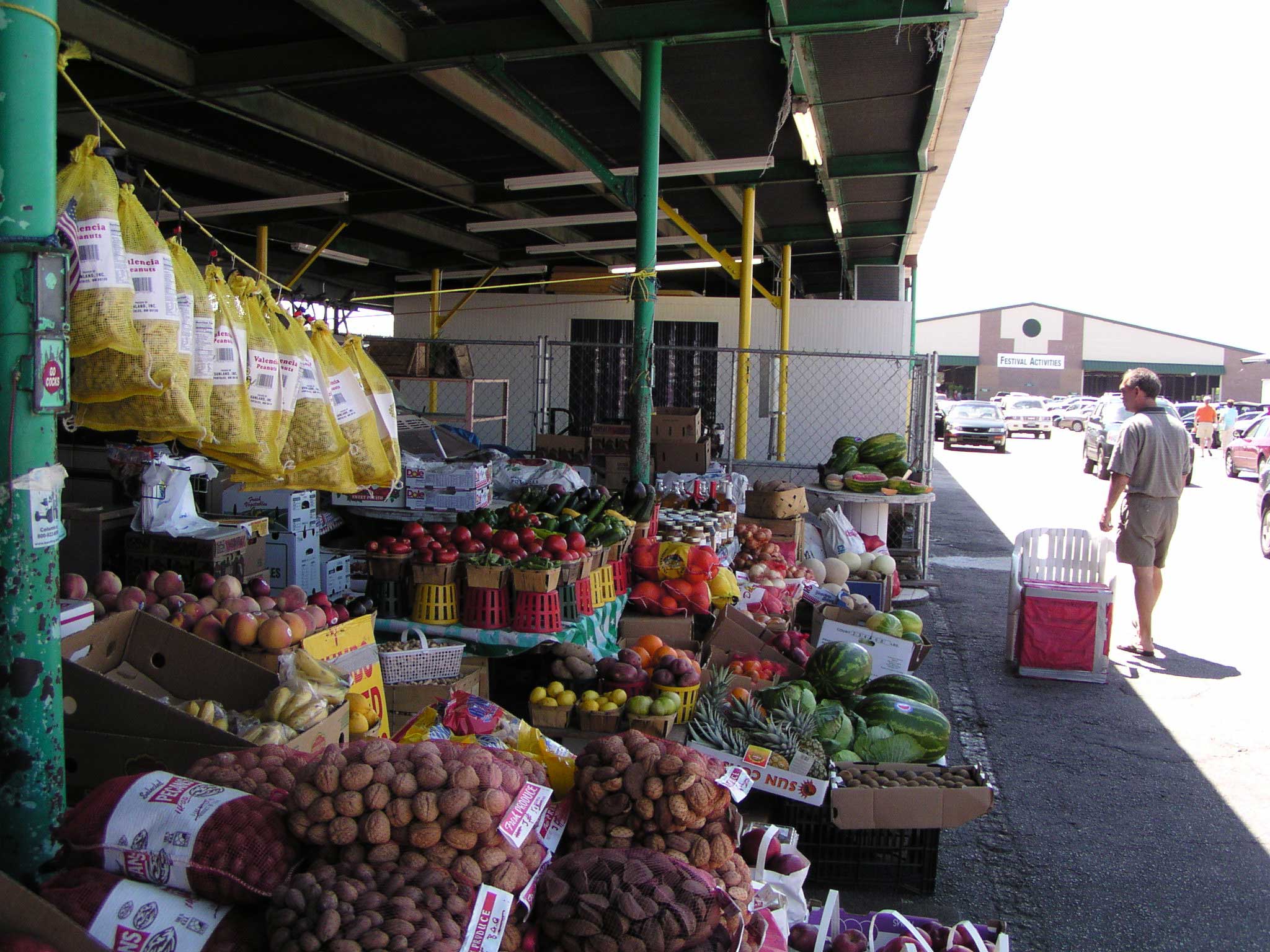
Economy in context
Produce displayed at a State Farmers Market stall in Columbia, South Carolina, with a shopper walking beside it.

A market price coordinates many separate decisions

Each buyer and seller arrives with different constraints and willingness to trade. The market model combines those individual plans into demand, supply, and one equilibrium benchmark.

Use this visual to see
Connect the supply-and-demand intersection to the decentralized choices visible in a working market.
What it cannot show
A photograph cannot show the full demand and supply schedules, prove that the observed price is an equilibrium, or reveal transactions that did not occur.

Use a four-step market change

  1. Name the market and axes.
  2. Identify the determinant that changed.
  3. Shift only the affected curve.
  4. Compare the old and new intersections for price and quantity.
  5. If both curves shift, evaluate price and quantity directions separately.

Keep these three ideas

  • Equilibrium requires quantity demanded to equal quantity supplied.
  • Shortages create upward price pressure; surpluses create downward pressure.
  • A curve shift changes equilibrium; simultaneous shifts may make one result indeterminate.

Basic economic concepts review

The unit moves from individual tradeoffs to an economy-wide frontier and then to market exchange. In every model, identify the constraint, the variables held constant, and the mechanism that changes the outcome.

Recognize immediately

  • State opportunity cost in units of the good forgone.
  • Distinguish movement along a curve from a shift of the curve.
  • Calculate comparative advantage from opportunity cost, not total output.
  • Use shortage and surplus to explain pressure toward equilibrium.
  • Treat efficiency and equity as different questions.

Practice AP Macroeconomics in the real test engine.

Free practice set: timed, the same engine as our full-length tests, every answer explained.