AP Physics C: E&M Unit 1: Electric Charges, Fields, and Gauss’s Law Notes

Introduction

Electric interactions begin with conserved, signed charge; Coulomb superposition builds forces and fields, while flux and Gauss’s law connect a closed surface to the charge it encloses.

Keep three objects separate: source charges create a field, a test charge samples that field, and a chosen system boundary determines which charge is conserved or enclosed. Vector direction comes from geometry and charge sign; magnitudes alone cannot describe an electric interaction.

For discrete charges, add Coulomb contributions as vectors. For continuous charge, replace the sum by a componentwise integral. Gauss’s law is always true for a closed surface, but it becomes a shortcut for the field only when spherical, cylindrical, or planar symmetry makes the surface integral reducible.

Charge and force

use signed sources, separation vectors, and superposition

Charging

track transferred charge across an explicit system boundary

Field and distributions

replace force-per-charge sums with vector integrals

Flux and Gauss’s law

connect oriented surface area to enclosed charge

Current exam guidance: Aligned to the current 2026–27 AP Physics C: Electricity and Magnetism framework, with calculus-based field, circuit, and induction models, explicit assumptions, and experimental reasoning.

8.1

Electric Charge and Electric Force

How do signed charges and geometry determine the net electrostatic force?

Short answer

Each source charge contributes an inverse-square force along its separation line, and the net force is the vector sum of those pairwise interactions.

Know firstVector components · Newton’s laws · Inverse-square relationships

Separate magnitude from direction

Charge is measured in coulombs and occurs in integer multiples of the elementary charge $e$ . For point charges, Coulomb’s law gives the force on charge 1 due to charge 2. Its magnitude is $k_e|q_1q_2|/r^2$ ; its line of action joins the charges. In vacuum, $k_e=1/(4\pi\epsilon_0)$ ; a material’s permittivity changes the ideal interaction by accounting for its polarization response. Like signs repel and unlike signs attract. Treat that verbal sign rule as direction logic rather than calling a magnitude negative.

With several sources, calculate every force on the same target charge and add components. Do not compare source-charge sizes and conclude that one member of an interaction pair feels more force: Newton’s third law still gives $\vec F_{1\leftarrow2}=-\vec F_{2\leftarrow1}$ . Quantitative course problems normally keep the discrete sum to four or fewer charges unless symmetry reduces the work. The point-charge model also applies outside a spherically symmetric distribution, but not automatically to overlapping or irregular extended bodies. Electric interaction dominates gravity between elementary charged particles, while gravity can dominate neutral macroscopic matter because positive and negative charge nearly cancel.

Physics model

Separation controls electric-force magnitude

Move a +2 μC point charge and a −3 μC point charge while their signs stay fixed. Their equal-and-opposite attractive forces follow the inverse square of center-to-center separation.

Charge separation2 m

Separation: 2 m
Force magnitude: 13.482 mN
Interaction: attractive

positive chargenegative chargeforce vectorscenter separation

F_e=k\frac{|q_1q_2|}{r^2}

Read this figure without the graphic

A positive charge sits left of a negative charge. Equal green force arrows point toward one another, and a center-to-center measure marks their separation.

Current quantity	Value
Separation	2 m
Force magnitude	13.482 mN
Interaction	attractive
Model relation	$F_e=k\frac{\|q_1q_2\|}{r^2}$

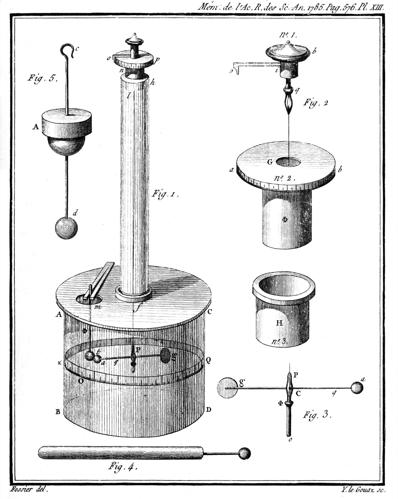
Coulomb’s 1784 drawing of a torsion balance with a suspended arm and charged spheres inside a glass enclosure. — Coulomb turned electric force into an angular measurement
A charged sphere deflects the suspended arm, while the twisted fiber supplies a restoring torque. Comparing equilibrium angles at different separations converts an invisible electric interaction into measurable mechanical evidence.
Use this visual to see
Connect Coulomb’s inverse-square force law to the equilibrium measurement that can test it.
What it cannot show
The drawing shows the tall enclosure, suspension fiber, rotating arm, and nearby spheres, but it supplies no charge values, separation scale, torsion constant, or numerical force measurement.

Resolve one attractive interaction

System: Two point charges in otherwise empty space.
Frame: The x-axis points from charge 1 at $x=0$ toward charge 2 at $x=0.30\ \mathrm{m}$ .
Assumptions: Charge sizes are negligible relative to separation and the medium is approximated as vacuum.
Givens: $q_1=+2.0\ \mathrm{nC}$ , $q_2=-8.0\ \mathrm{nC}$ , and $k_e=9.0\times10^9\ \mathrm{N\,m^2/C^2}$ .

Use the center-to-center separation $r=0.30\ \mathrm{m}$ .
Compute $F=k_e|q_1q_2|/r^2=1.60\times10^{-6}\ \mathrm{N}$ .
Unlike signs attract, so the force on charge 1 points in $+x$ .
The force on charge 2 has the same magnitude and points in $-x$ .

Result

\vec F_{1\leftarrow2}=+1.60\times10^{-6}\hat i\ \mathrm{N},\qquad \vec F_{2\leftarrow1}=-\vec F_{1\leftarrow2}

Units:

k_eq_1q_2/r^2

reduces to newtons.

Boundary cases

$r=0$ is excluded from the point-charge model.
At distances much larger than a spherical source radius, the exterior field has the same form as a point charge.

The positive charge lies left of the negative charge, so attraction pulls the left charge right and the right charge left with equal force magnitude.

Build each vector contribution

Step	Question	Record
source	Which charge produces this contribution?	$q_s$ and its position
target	Which charge experiences the force?	$q_t$
geometry	What is the source-to-target direction?	$\hat r_{s\to t}$
magnitude	How large is the interaction?	$k_e\|q_sq_t\|/r^2$
sum	What acts on the target?	$\sum\vec F_i$ in components

Audit a Coulomb-force sum

Sketch every charge and declare axes.
Choose one target charge.
For each source, find separation and attraction or repulsion direction.
Resolve the force into components before adding.
Check units, inverse-square scaling, and the third-law partner.

Keep these three ideas

Coulomb force is inverse-square and directed along the separation line.
Superposition adds vectors on one target.
Interaction partners are equal and opposite even for unequal charges.

8.2

Conservation of Electric Charge and the Process of Charging

How can an object become charged without creating or destroying charge?

Short answer

Charging transfers or redistributes existing charge; the total remains constant when the system boundary includes every body that exchanges charge.

Know firstAtomic charge carriers · System boundaries · Conservation laws

A charge ledger depends on the boundary

In ordinary solid materials, electrons move between or within objects while protons remain bound in nuclei. Friction and contact transfer electrons. Polarization separates positive and negative regions without necessarily changing net charge. Induction combines polarization with a carefully ordered connection to ground so an object can retain net charge without touching the external charged body.

Charge conservation applies to an isolated system. If Earth supplies or receives electrons, the object alone is open to charge transfer; object plus Earth is the larger conserved system. Quantization gives $Q=Ne$ , although macroscopic charge usually contains so many elementary charges that a continuous value is an excellent approximation.

Physics model

Charging moves charge without changing the system total

Move signed charge between sphere A, initially +8 nC, and sphere B, initially −2 nC. The individual charges change while the closed two-sphere total remains +6 nC.

Signed transfer A → B3 nC

Sphere A: +5 nC
Sphere B: +1 nC
System total: +6 nC

sphere Asphere Btransferred chargesystem boundary

\begin{aligned}Q_{A,f}&=Q_{A,i}-\Delta q\\Q_{B,f}&=Q_{B,i}+\Delta q\end{aligned}

Read this figure without the graphic

Two spheres sit inside one system boundary. A directed transfer marker connects them while signed sphere totals and the unchanged system total appear above the diagram.

Current quantity	Value
Sphere A	+5 nC
Sphere B	+1 nC
System total	+6 nC
Model relation	$\begin{aligned}Q_{A,f}&=Q_{A,i}-\Delta q\\Q_{B,f}&=Q_{B,i}+\Delta q\end{aligned}$

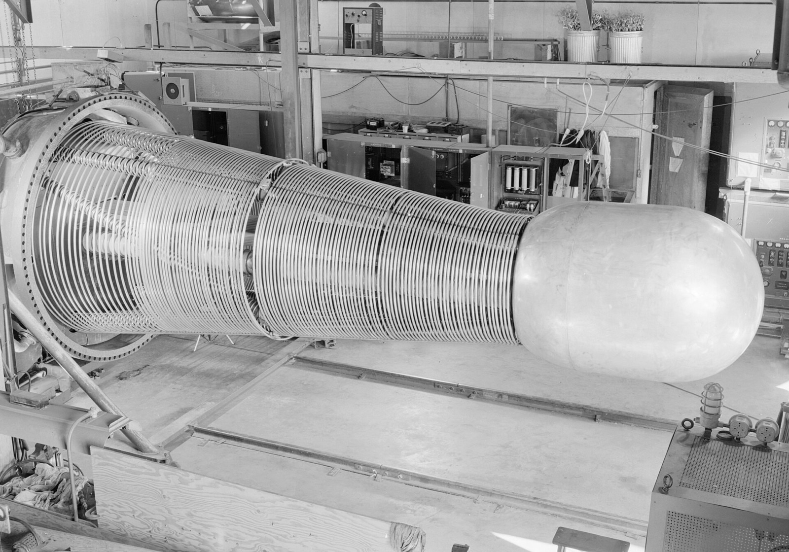
Large Van de Graaff electrostatic generator photographed at Lawrence Berkeley Laboratory in 1948. — A Van de Graaff generator separates and accumulates charge
The generator transports charge onto a large conducting terminal instead of creating net charge from nothing. Its growing potential reflects charge separation between the terminal, the machine, and the surrounding environment.
Use this visual to see
Show conservation of charge within a real process that transfers charge between parts of a system.
What it cannot show
The photograph establishes the scale and conducting terminal of the apparatus but does not reveal charge sign, transferred charge, belt motion, leakage rate, electric field, or potential.

Track a transfer without losing charge

System: Two initially neutral isolated objects A and B.
Frame: A charge ledger; spatial axes are not needed.
Assumptions: Only electrons transfer between A and B, and no charge reaches the surroundings.
Givens: Electrons carrying $3.0\ \mathrm{nC}$ move from A to B.

A loses negative charge, so $Q_A=+3.0\ \mathrm{nC}$ .
B gains the same negative charge, so $Q_B=-3.0\ \mathrm{nC}$ .
Add the final charges and compare with the initial total.
Divide the transferred magnitude by $e$ to estimate $1.87\times10^{10}$ electrons.

Result

Q_{A,f}+Q_{B,f}=+3.0\ \mathrm{nC}-3.0\ \mathrm{nC}=0=Q_{A,i}+Q_{B,i}

Units: Charge is in coulombs; the carrier count is dimensionless.

Boundary cases

If B is grounded, the two-object total need not remain fixed because Earth is outside that boundary.
Polarization can change the surface distribution while net charge remains zero.

Three nanocoulombs of negative charge leave A and enter B, producing equal positive and negative final charges and an unchanged two-object total.

Distinguish charging processes

Process	What changes?	Boundary warning
friction or contact	electrons transfer between materials	include both bodies
polarization	bound or mobile charge redistributes	net object charge may stay zero
induction with grounding	Earth exchanges electrons after polarization	include Earth for conservation
discharge	excess charge leaves through a conducting path	include the receiving body

Read an induction sequence

Name the object, external charge, and ground.
Track electron motion at each numbered state.
Do not remove the external charge before disconnecting ground if a residual charge is intended.
Choose a conserved system that includes every charge-transfer path.
Check final sign by recounting electrons, not by memorized slogans.

Keep these three ideas

Charging transfers or redistributes existing charge.
Grounding changes which system is isolated.
Induction requires the sequence of polarization, grounding, and disconnection.

8.3

Electric Fields

How does a source configuration assign force-per-charge throughout space?

Short answer

The electric field is the vector force a sufficiently small positive test charge would experience per unit charge, independent of that test charge’s sign and mass.

Know firstCoulomb force · Vector superposition · Limits

Define the field before placing the particle

At a field point, $\vec E=\vec F/q_0$ in the limit that a positive test charge $q_0$ does not disturb the sources. A point source gives $\vec E=k_eq\hat r/r^2$ , directed away from positive charge and toward negative charge. Once $\vec E$ is known, a particle feels $\vec F=q\vec E$ ; a negative particle therefore accelerates opposite the field when electric force is the only force.

Field contributions superpose linearly. Field lines are a drawing convention: their tangents show direction and their spacing suggests strength. They do not cross at a regular point and are not guaranteed particle paths. Exclude a point charge’s self-field at its own location. In electrostatic equilibrium a conductor has zero field inside its material and exterior field normal to its surface; an insulator can retain volume charge and a nonzero interior field.

Physics model

Electric fields superpose as vectors

Move a field point between +1 μC at x = −2 m and −1 μC at x = +2 m. Both contributions point right between the sources, so their vector magnitudes add.

Field-point position0 m

From + source: 2.247 kN/C right
Toward − source: 2.247 kN/C right
Net field: 4.494 kN/C right

field from + sourcefield from − sourcenet electric fieldfield point

\vec E(\vec r)=\frac{1}{4\pi\epsilon_0}\sum_i\frac{q_i(\vec r-\vec r_i)}{|\vec r-\vec r_i|^3}

Read this figure without the graphic

A field point lies between a positive source on the left and a negative source on the right. Both source contributions and their net vector point to the right.

Current quantity	Value
From + source	2.247 kN/C right
Toward − source	2.247 kN/C right
Net field	4.494 kN/C right
Model relation	$\vec E(\vec r)=\frac{1}{4\pi\epsilon_0}\sum_i\frac{q_i(\vec r-\vec r_i)}{\|\vec r-\vec r_i\|^3}$

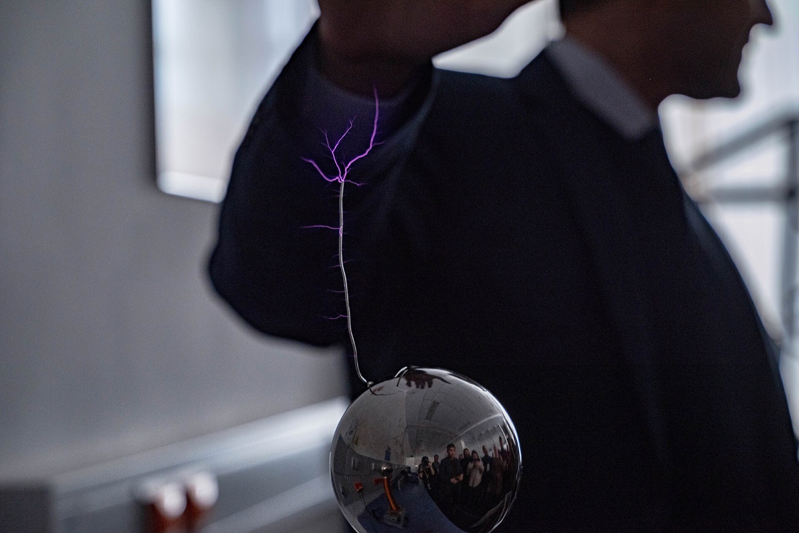
Bright branching electric spark crosses an air gap between conducting laboratory electrodes. — A sufficiently strong electric field can make air conduct
Ordinary air is insulating, but a sufficiently strong electric field accelerates charges enough to ionize molecules and create a conducting path. The luminous channel appears after breakdown begins.
Use this visual to see
Connect electric-field strength to charge acceleration and the onset of electrical breakdown in air.
What it cannot show
The photograph shows a bright, branching discharge between conductors but provides no electric-field magnitude, field-vector map, electrode separation, voltage, charge density, or time development.

Use symmetry without discarding components

System: Two equal positive point charges and an empty field point.
Frame: Charges $+q$ lie at $(\pm a,0)$ ; the field point lies at $(0,y)$ .
Assumptions: Point charges are fixed and the field point excludes the sources.
Givens: Each source-to-point distance is $R=\sqrt{a^2+y^2}$ .

Write each field with magnitude $k_eq/R^2$ .
Resolve each vector along x and y.
The horizontal components cancel by mirror symmetry.
The vertical components add, each contributing $k_eqy/R^3$ .

Result

\vec E(0,y)=\frac{2k_eqy}{(a^2+y^2)^{3/2}}\hat j

Units: Electric field has units N/C, equivalently V/m.

Boundary cases

$\vec E(0,0)=0$ although the potential there need not be zero.
As $|y|\gg a$ , the pair approaches the field of total charge $2q$ .

At a point on the perpendicular bisector, equal horizontal field components oppose and equal vertical components reinforce.

Keep source, field, and force distinct

Quantity	Depends on	Direction
source field $\vec E$	source charge and field-point geometry	defined using a positive test charge
particle force $\vec F$	$q\vec E$	with $\vec E$ for $q>0$ , opposite for $q<0$
field-line tangent	authored field representation	local field direction
particle path	initial velocity plus all forces	not generally a field line

Find a net electric field

Mark the field point separately from every source.
Draw each source-to-field-point vector.
Determine each field direction from source sign.
Resolve and add components.
Apply $\vec F=q\vec E$ only after the source field is complete.

Keep these three ideas

Electric field is source-defined force per positive test charge.
A negative charge feels force opposite the field.
Field lines encode direction and strength but are not particle paths.

8.4

Electric Fields of Charge Distributions

How does an extended charge distribution build an electric field?

Short answer

Replace discrete source charge by $dq$ , express its separation and direction from the integration geometry, and integrate the surviving field components over the distribution.

Know firstElectric-field superposition · Integral calculus · Linear, surface, and volume density

Integrate vectors, not just charge

Use $dq=\lambda\,dl$ , $dq=\sigma\,dA$ , or $dq=\rho\,dV$ according to how charge occupies space. Each element contributes $d\vec E=k_e(dq/R^2)\hat R$ , where $\vec R$ points from the source element to the field point. The integration variable locates the source; $R$ is the source-to-point separation. Giving both the same symbol hides the geometry and usually corrupts the denominator.

Symmetry can cancel paired components before integration, but it cannot turn an arbitrary distribution into a point charge. The quantitative course boundary includes infinite uniform wire or cylinder fields off axis, a ring on axis, a semicircular arc or portion at its center, and finite-line fields on axis or the perpendicular bisector. Far from a localized distribution, a correct result should approach the field of its total charge.

Physics model

A continuous distribution adds infinitesimal field contributions

Move along the axis of a uniformly charged ring with Q = +2 μC and R = 2 m. Paired transverse components cancel while the axial components add.

Axis distance2 m

Axis distance: 2 m
Ring radius: 2 m
Axial field: 1.589 kN/C

charged ringpaired element pathsaxial fieldobservation point

E_z=\frac{kQz}{(z^2+R^2)^{3/2}}

Read this figure without the graphic

A charged ring is shown edge-on with paired source elements joined to a point on its axis. Sideways components cancel and one axial field vector remains.

Current quantity	Value
Axis distance	2 m
Ring radius	2 m
Axial field	1.589 kN/C
Model relation	$E_z=\frac{kQz}{(z^2+R^2)^{3/2}}$

Build the axial field of a charged ring

System: A uniformly charged thin ring of radius $a$ and total charge $Q$ .
Frame: The ring lies in the xy-plane; the field point is $(0,0,z)$ .
Assumptions: The ring is thin, stationary, and uniformly charged.
Givens: $dq=(Q/2\pi)\,d\phi$ and every element is distance $R=\sqrt{a^2+z^2}$ from the point.

Pair diametrically opposite elements so transverse field components cancel.
The surviving axial component is $dE_z=k_e z\,dq/R^3$ .
Because $z$ and $R$ are constant around the ring, integrate $dq$ to $Q$ .
Check the center and far-field limits.

Result

\vec E(z)=\frac{k_eQz}{(z^2+a^2)^{3/2}}\hat k

Units:

k_eQz/(z^2+a^2)^{3/2}

has units N/C.

Boundary cases

$E_z(0)=0$ by symmetry.
For $|z|\gg a$ , $E_z\to k_eQz/|z|^3$ , the point-charge result with the correct axial sign.

Opposite ring elements cancel sideways; every axial component points the same way, leaving one integral over the total charge.

Translate density into charge

Distribution	Differential charge	Integration measure
line or arc	$dq=\lambda\,dl$	length
surface	$dq=\sigma\,dA$	area
volume	$dq=\rho\,dV$	volume
uniform ring	$dq=(Q/2\pi)d\phi$	angle after radius is fixed

Set up a distribution integral

Draw one source element and the field point.
Write $dq$ in one integration variable.
Construct the separation vector $\vec R$ .
Use symmetry to identify canceled and surviving components.
Integrate over the actual source limits, then test center and far-field behavior.

Keep these three ideas

Convert density to $dq$ using the source geometry.
Integrate field components with a distinct separation vector.
Center and far-field limits expose many setup errors.

8.5

Electric Flux

How does an electric field pierce an oriented surface?

Short answer

Electric flux is the signed surface integral of the field component normal to an oriented area, not the amount of field or charge physically flowing through it.

Know firstDot products · Surface normals · Riemann sums and surface integrals

Orientation gives flux its sign

A small oriented patch has area vector $d\vec A=\hat n\,dA$ . Its contribution is $d\Phi_E=\vec E\cdot d\vec A$ . For an open surface, choose one of the two possible normal directions and keep it fixed. For a closed surface, the normal is outward by convention and the integral is written $\oint$ .

A uniform field through a flat area gives $\Phi_E=EA\cos\theta$ , where $\theta$ is the angle between the field and the normal—not between the field and the plane. Positive and negative patch contributions can cancel. In a uniform field, any closed surface has zero net flux even though the local field and individual face fluxes are nonzero.

Physics model

Flux measures the normal component through an oriented area

Rotate a 0.040 m² flat surface in a uniform 0.60 kN/C electric field. Signed flux follows the component of the field along the chosen area normal.

Field-to-normal angle60 °

Angle: 60°
Normal field: 0.3 kN/C
Electric flux: 12 N·m²/C

electric fieldoriented surfacearea normalangle θ

\Phi_E=\int_S\vec E\cdot d\vec A=EA\cos\theta

Read this figure without the graphic

Parallel electric-field arrows cross an oriented surface. The area normal rotates with the surface, and the marked angle determines the signed flux.

Current quantity	Value
Angle	60°
Normal field	0.3 kN/C
Electric flux	12 N·m²/C
Model relation	$\Phi_E=\int_S\vec E\cdot d\vec A=EA\cos\theta$

Use the area vector directly

System: A flat open surface in a uniform electric field.
Frame: Cartesian components define both field and chosen area normal.
Assumptions: The field is constant over the surface.
Givens: $\vec E=(3,4,0)\ \mathrm{N/C}$ and $\vec A=(2,-1,0)\ \mathrm{m^2}$ .

Use the area vector rather than separately finding $A$ and $\theta$ .
Take the dot product: $3(2)+4(-1)+0(0)$ .
Retain the sign set by the chosen normal.
Check units as field times area.

Result

\Phi_E=\vec E\cdot\vec A=2\ \mathrm{N\,m^2/C}

Units: Electric flux is measured in N·m²/C.

Boundary cases

Reversing the open-surface normal changes the sign.
A field tangent to every patch has zero flux through that surface.

The positive x contribution is six and the negative y contribution is four, leaving signed flux two.

Read a patchwise flux ledger

Field relative to outward normal	$\vec E\cdot d\vec A$	Patch contribution
outward	positive	positive flux
inward	negative	negative flux
tangent	zero	zero flux
varying direction or magnitude	varies	integrate or sum patches

Evaluate flux without an angle trap

Mark whether the surface is open or closed.
Draw or state the normal orientation.
Write $\vec E\cdot\hat n$ for each region.
Integrate over the surface or sum well-defined patches.
Check sign, units, and cancellation between opposite faces.

Keep these three ideas

Flux integrates the normal field component over oriented area.
Closed-surface normals point outward.
Nonzero field can coexist with zero net closed flux.

8.6

Gauss’s Law

When can a closed-surface flux law determine the local electric field?

Short answer

Gauss’s law always fixes total closed flux from enclosed charge, but it isolates field magnitude only when source symmetry makes the integrand uniform or zero on chosen surface patches.

Know firstElectric flux · Charge density · Spherical, cylindrical, and planar symmetry

The law is general; the shortcut is not

Gauss’s law, the integral form of the first Maxwell equation, states $\oint_S\vec E\cdot d\vec A=Q_{enc}/\epsilon_0$ for every closed surface. The right side includes only charge inside that surface. External charges can create a strong, nonuniform field on the surface, but their total contribution to closed flux is zero because their field lines enter and leave in equal net amount.

To solve directly for $E$ , the physical source—not the imagined Gaussian surface—must have enough symmetry. Spherical sources use concentric spheres, infinite line or cylindrical sources use coaxial cylinders, and infinite sheets use pillboxes. On useful patches, symmetry must establish the field direction and constant magnitude. An irregular surface can still give total flux, but usually not the field at each point.

Physics model

Symmetry turns a flux integral into an electric field

Change the Gaussian radius around a uniformly charged sphere with Q = +6 nC and R = 2 m. Enclosed charge grows with volume inside and remains 6 nC outside.

Gaussian radius2 m

Enclosed charge: 6 nC
Field magnitude: 13.482 N/C
Region: source surface

source chargeGaussian surfaceenclosed chargeradial field

\oint_S\vec E\cdot d\vec A=\frac{Q_{enc}}{\epsilon_0}

Read this figure without the graphic

A dashed Gaussian sphere is concentric with a uniformly charged source sphere. Enclosed source charge and radial field arrows change with Gaussian radius.

Current quantity	Value
Enclosed charge	6 nC
Field magnitude	13.482 N/C
Region	source surface
Model relation	$\oint_S\vec E\cdot d\vec A=\frac{Q_{enc}}{\epsilon_0}$

Reduce the integral for a centered point charge

System: A point charge $q$ enclosed by a spherical Gaussian surface of radius $r$ .
Frame: The charge is at the sphere center; outward radial direction is positive.
Assumptions: The field is electrostatic and vacuum permittivity applies.
Givens: $q=2.0\ \mathrm{nC}$ and $\epsilon_0=8.8541878128\times10^{-12}\ \mathrm{C^2/(N\,m^2)}$ .

Spherical symmetry makes $\vec E$ radial and its magnitude constant on the sphere.
Therefore $\vec E\cdot d\vec A=E\,dA$ .
Integrate area to obtain $E(4\pi r^2)=q/\epsilon_0$ .
The total flux is independent of the chosen radius.

Result

\Phi_E=\frac{q}{\epsilon_0}=2.26\times10^2\ \mathrm{N\,m^2/C},\qquad E=\frac{q}{4\pi\epsilon_0r^2}

Units:

q/\epsilon_0

has units N·m²/C; dividing by area gives N/C.

Boundary cases

A closed surface that does not enclose the charge has zero net flux but may have nonzero field.
A Gaussian surface passing through a point charge is invalid because the field is singular there.

A centered point charge produces equal radial field magnitude everywhere on a sphere, so flux is field magnitude times the sphere area.

Match source symmetry to a Gaussian surface

Physical source	Useful surface	Integral reduction
spherical or point charge	concentric sphere	$E(4\pi r^2)$
infinite line or cylinder	coaxial cylinder	$E(2\pi rL)$ when end flux is zero
infinite plane	pillbox	$2EA$ for equal fields on both faces
arbitrary source	any closed surface	total flux known; local $E$ generally not isolated

Decide whether Gauss’s law is a field-solving tool

Identify the physical source symmetry.
Choose a closed surface aligned with that symmetry.
State why $\vec E$ is parallel, perpendicular, or constant on each patch.
Compute $Q_{enc}$ , integrating density if necessary.
Apply the law and test inside, outside, and far-field limits.

Keep these three ideas

Gauss’s law relates closed flux to enclosed charge.
External charge affects local field but contributes zero net closed flux.
Only source symmetry permits a direct reduction to field magnitude.

Cumulative review

Electric charges and fields review

The unit progresses from pair interactions to a field defined throughout space, then from local field samples to the global flux of a closed surface. Every valid solution preserves vectors, source geometry, and the chosen system or surface boundary.

Recognize immediately

Choose the source point, field point, coordinate axes, and excluded singular locations before calculating.
Add force and field contributions as vectors; use charge sign to determine direction.
Use $dq=\lambda\,dl$ , $dq=\sigma\,dA$ , or $dq=\rho\,dV$ and integrate only the components that survive symmetry.
Distinguish an open-surface flux calculation from a closed-surface Gauss-law argument.
Use Gauss’s law to solve for $E$ only when symmetry fixes both field direction and magnitude behavior on the chosen surface.

Introduction

Separate magnitude from direction

Coulomb turned electric force into an angular measurement

Resolve one attractive interaction

Boundary cases

Build each vector contribution

Audit a Coulomb-force sum

Keep these three ideas

A charge ledger depends on the boundary

A Van de Graaff generator separates and accumulates charge

Track a transfer without losing charge

Boundary cases

Distinguish charging processes

Read an induction sequence

Keep these three ideas

Define the field before placing the particle

A sufficiently strong electric field can make air conduct

Use symmetry without discarding components

Boundary cases

Keep source, field, and force distinct

Find a net electric field

Keep these three ideas

Integrate vectors, not just charge

Build the axial field of a charged ring

Boundary cases

Translate density into charge

Set up a distribution integral

Keep these three ideas

Orientation gives flux its sign

Use the area vector directly

Boundary cases

Read a patchwise flux ledger

Evaluate flux without an angle trap

Keep these three ideas

The law is general; the shortcut is not

Reduce the integral for a centered point charge

Boundary cases

Match source symmetry to a Gaussian surface

Decide whether Gauss’s law is a field-solving tool

Keep these three ideas

Electric charges and fields review

Recognize immediately

Practice AP Physics C: E&M in the real test engine.